In the last post I presented a way to do Bayesian networks with pymc and use them to impute missing data. This time I benchmark the accuracy of this method on some artificial datasets.
Datasets
In the previous posts I showed the imputation of boolean missing data, but the same method works for categorical features of any cardinality as well as continuous ones (except in the continues case additional prior knowledge is required to specify the likelihood). Nevertheless, I decided to test the imputers on purely boolean datasets because it makes the scores easy to interpret and the models quick to train.
To make it really easy on the Bayesian imputer, I created a few artificial datasets by the following process:
define a Bayesian network
sample variables corresponding to conditional probabilities describing the network from their priors (once)
fix the parameters from step 2. and sample the other variables (the observed ones) repeatedly
With data generated by the same Bayesian network that we will fit to it, we’re making it as easy on pymc as possible to get a good score. Mathematically speaking, the bayesian model is the way to do it. Anything less than optimal performance can only be due to a bug or pymc underfitting (perhaps from too few iterations).
The first dataset used is based on the famous wet sidewalk - rain - sprinkler network as seen in the wikipedia article on Bayesian networks.
For each of these networks I would generate a dataframe with 10, 50, 250, 1250 or 6250 records and drop (replace with -1) a random subset of 20% or 50% of values in each column. Then I would try to fill them in with each model and score the model on accuracy. This was repeated 5 times for each network and data size and the accuracy reported is the mean of the 5 tries.
Models
The following models were used to impute the missing records:
most frequent - a dummy model that predicts most frequent value per dataframe column. This is the absolute baseline of imputer performance, every model should be at least as good as this.
xgboost - a more ambitious machine learning-based baseline. This imputer simply trains an XGBoost Classifier for every column of the dataframe. The classifier is trained only on the records where the value of that column is not missing and it uses all the remaining columns to predict that one. So, if there are n columns - n classifiers are trained, each using n - 1 remaining columns as features.
MAP fmin_powell - a model constructed the same way as the DuckImputer model from the previous post. Actually, it’s a different model for each dataset, but the principle is the same. You take the very same Bayesian network that was used to create the dataset and fit it to the dataset. Then you predict the missing values using MAP with ‘method’ parameter set to ‘fmin_powell’.
MAP fmin - same as above, only with ‘method’ set to ‘fmin’. This one actually performed so poorly, (no better than random and worse than most frequent) and was so slow that I quickly dropped it from the benchmark
MCMC 500, MCMC 2000, MCMC 10000 - same as the MAP models, except for the last step. Instead of finding maximum a posteriori for each variable directly using the MAP function, the variable is sampled n times from the posterior using MCMC, and the empirically most common value is used as the prediction. Three versions of this model were used - with 500, 2000 and 10000 iterations for burn-in repectively. After burn-in, 200 samples were used each time.
Results
Let’s start with the simplest network:
Rain-Sprinkler-Wet Sidewalk benchmark (20% missing values). Mean imputation accuracy from 5 runs vs data size.
Average fitting time in seconds. Beware log scale!
XGBoost comes out on top, bayesian models do poorly, apparently worse than even most frequent imputer. But variance in scores is quite big and there is not much structure in this dataset anyway, so let’s not lose hope. MAP fmin_powell is particularly bad and terribly slow on top of that, dropping it from further benchmarks.
Let’s try a wider dataset - the cancer network. This one has more structure - that the bayesian network knows up front and xgboost doesn’t - which should give bayesian models an edge.
Cancer network imputation accuracy. 20% missing values
Cancer network imputation time.
That’s more like it! MCMC wins when records are few, but deteriorates when data gets bigger. MCMC models continue to be horribly slow.
And finally, the biggest (27 features!), car insurance network.
Car insurance network imputation accuracy. 20% missing values
Car insurance network imputation time.
Qualitatively same as the cancer network case. It’s worth pointing out that in this case, the Bayesian models achieve at 50 records a level of accuracy that XGBoost doesn’t match until shown more than a thousand records! Still super slow though.
Conclusions
What have we learned?
Bayesian models do relatively better when data is wide (more columns). This was expected. Wide data means bigger network, means there is more information implicit in the network structure. This is information that we hardcode into the Bayesian model, information that XGBoost doesn’t have.
Bayesian models do relatively better when data is short (less records). This was also expected, for the same reason. When data is short, the information contained in the network counts for a lot. With more records to train on, this advantage gets less important.
pymc’s MAP does poorly in terms of accuracy and is terribly slow, slower than MCMC. This one is a bit of a mystery.
For MCMC, longer burn-in gets better results, but takes more time. Duh.
MCMC model accuracy deteriorates as data gets bigger. I was surprised when I saw it, but it hindsight it’s clear that it would be the case. Bigger data means more missing values, means higher dimensionality of the space MCMC has to explore, means it would take more iterations for MCMC to reach a high likelihood configuration. This could be alleviated if we first learned the most likely values of the parameters of the network and then used those to impute the missing values one record at a time.
XGBoost rocks.
Overall, I count this experiment as a successful proof of concept, but of very limited usefulness in its current form. For any real world application one would have to redo it using some other technology. pymc is just not up to the task.
This is the first of two posts about Bayesian networks, pymc and missing data. In the first post I will show how to do Bayesian networks in pymc* and how to use them to impute missing data. This part is boring and slightly horrible. In the second post I investigate how well it actually works in practice (not very well) and how it compares to a more traditional machine learning approach (poorly). Feel free to go straight to the second post, it has plots in it.
This post assumes that the reader is already familiar with both bayesianism and pymc. If you aren’t, I recommend that you check out the fantastic Bayesian Methods For Hackers.
* technically, everything in pymc is a Bayesian network, I know
The problem
We have observed 10 animals and noted 3 things about each of them:
- does it swim like a duck?
- does it quack like a duck?
- is it, in fact, a duck?
12345678
importpandasaspd# we use 1 and 0 to represent True and False for reasons that will become clear laterfull=pd.DataFrame({'swims_like_a_duck':[0,0,0,0,1,1,1,1,1,1],'quacks_like_a_duck':[0,1,0,1,0,1,0,1,0,1],'duck':[0,0,0,0,0,1,0,1,0,1]})
It is easy to notice that in this dataset an animal is a duck if and only if it both swims like a duck and quacks like a duck. So far so good.
But what if someone forgets to write down whether the duck number 10 did any quacking or whether the animal number 9 was a duck at all? Now we have missing data. Here denoted by -1
This tells us about the last animal that it is a duck, but the information about swimming and quacking is missing. Nevertheless, having established the rule
we can infer that the values of swims_like_a_duck and quacks_like_a_duck must both be 1 for this animal.
This is what we will try to do here - learn the relationship between the variables and use it to fill in the missing ones.
The Bayesian solution
To be able to attack this problem, let’s make one simplifying assumption. Let’s assume that we know the causal structure of the problem upfront. That is - we know that swimming and quacking are independent random variables, while being a duck is a random variable that potentially depends on the other two.
This is the situation described by this Bayesian network:
This network is fully characterised by 6 parameters - prior probabilities of swimming and quacking -
$P(swims)$, $P(quacks)$
- and conditional probability of being a duck given values of the other 2 variables -
$P(duck \mid swims \land quacks)$,
$P(duck \mid \neg swims \land quacks)$
- and so on. We don’t know anything about the values of these parameters, other than they must be between $0$ and $1$. The bayesian thing to do in such situations is to model the unknown parameters as random variables of their own and give them uniform priors.
Thus, the network expands:
This is the network describing a single animal, but actually we have observations of many animals, so the full network would look more like this:
There is only one node corresponding to each of the 6 parameters, but there are as many ‘swims’ and ‘quacks’ and ‘duck’ nodes as there are records in the dataset.
Some of the variables are observed (orange), others aren’t (white), but we have specified priors for all the parent variables and the model is fully defined. This is enough to (via Bayes theorem) derive the formula for the posterior probability of every unobserved variable and the posterior distribution of every model parameter.
But instead of doing math, we will find a way to programmatically estimate all those probabilities with pymc. This way, we will have a solution that can be easily extended to arbitrarily complicated networks.
What could go wrong?
pymc implementation
Disclaimer: this is all hacky and inefficient in ways I didn’t realise it would be when I started working on it. pymc is not the right tool for the job, if you want to do this seriously, in a production environment you should look for something else. pymc3 maybe?
I will now demonstrate how to represent our quack-swim-duck Bayesian network in pymc and how to make predictions with it. pymc was confusing the hell out of me when I first started this project. I will be painstakingly explicit at every step of this tutorial to save the reader some of this confusion. Then at the end I will show how to achieve the same result with 1/10th as many lines of code using some utilities of my invention.
Let’s start with the unobserved variables:
1234567891011
importpymc# prior probabilities for swimming and quackingswim_prior=pymc.Uniform('P(swims)',lower=0,upper=1,size=1)quack_prior=pymc.Uniform('P(quacks)',lower=0,upper=1,size=1)# probability of being a duck conditional on swimming and quacking# (or not swimming and quacking etc.)p_duck_swim_quack=pymc.Uniform('P(duck | swims & quacks)',lower=0,upper=1,size=1)p_duck_not_swim_not_quack=pymc.Uniform('P(duck | not swims & not quacks)',lower=0,upper=1,size=1)p_duck_not_swim_quack=pymc.Uniform('P(duck | not swims & quacks)',lower=0,upper=1,size=1)p_duck_swim_not_quack=pymc.Uniform('P(duck | swims & not quacks)',lower=0,upper=1,size=1)
Now the observed variables. pymc requires that we use masked arrays to represent missing values:
# number of animal observationsn=len(with_missing)# with 'size=n' with tell pymc that 'swims' is actually a sequence of n Bernoulli variablesswims=pymc.Bernoulli('swims',p=swim_prior,observed=True,value=masked_swim_data,size=n)quacks=pymc.Bernoulli('quacks',p=quack_prior,observed=True,value=masked_quack_data,size=n)
And now the hard part. We have to construct a Bernoulli random variable ‘duck’, whose conditional probability given its parents is equal to a different random variable for very combination of values of the parents. That was a mouthful, but all it means is that there is a conditional probability table of ‘duck’ conditioned on ‘swims’ and ‘quacks’. This is literally the first example in every textbook on probabilistic models. And yet, there is no easy way to express this relationship with pymc. We are forced to roll our own custom function.
123456789101112131415161718192021222324252627
# auxiliary pymc variable - probability of duck@pymc.deterministicdefduck_probability(swims=swims,quacks=quacks,p_duck_swim_quack=p_duck_swim_quack,p_duck_not_swim_quack=p_duck_not_swim_quack,p_duck_swim_not_quack=p_duck_swim_not_quack,p_duck_not_swim_not_quack=p_duck_not_swim_not_quack):d=[]fors,qinzip(swims,quacks):if(sandq):d.append(p_duck_swim_quack)elif(sand(notq)):d.append(p_duck_swim_not_quack)elif((nots)andq):d.append(p_duck_not_swim_quack)elif((nots)and(notq)):d.append(p_duck_not_swim_not_quack)else:raiseValueError('this should never happen')returnnp.array(d).ravel()# AND FINALLYduck=pymc.Bernoulli('duck',p=duck_probability,observed=True,value=masked_duck_data,size=n)
If you’re half as confused reading this code as I was when I was first writing it, you deserve some explanations.
‘swims’ and ‘quacks’ are of type pymc.distributions.Bernoulli, but here we treat them like numpy arrays.
This is @pymc.deterministic’s doing. This decorator ensures that when this function is actually called it will be given swims.value and quacks.value as parameters - and these are indeed numpy arrays. Same goes for all the other parameters.
earlier we used a pymc random variable for the p parameter of a pymc.Bernoulli but now we’re using a function - duck_probability
Again, @pymc.deterministic. When applied to a function it returns an object of type pymc.PyMCObjects.Deterministic. At this point the thing bound to the name ‘duck_probability’ is no longer a function. It’s a pymc random variable. It has a value parameter and everything.
Ok, let’s put it all together in a pymc model:
12
# putting it all togethermodel=pymc.Model([swims,quacks,duck])
aaaand we’re done.
Not really. The network is ready, but there is still the small matter of extracting predictions out of it.
Making predictions with MAP
The obvious way to estimate the missing values is with a maximum a posteriori estimator. Thankfuly, pymc has just the thing - pymc.MAP. Calling .fit on a pymc.MAP object changes values of variables in place, so let’s print the values of some of our variables before and after fitting.
>>>pymc.MAP(model).fit()Warning:Stochasticswims's value is neither numerical nor array with floating-point dtype. Recommend fitting method fmin (default).
The two False bits - in ‘swims’ and ‘quacks’ have flipped to True and the values of the conditional probabilities have moved in the right direction! This is good, but unfortunately it’s not reliable. Even in this simple example pymc’s MAP rarely gets everything right like it did this time. To some extent it depends on the optimisation method used - e.g. pymc.MAP(model).fit(method='fmin') vs pymc.MAP(model).fit(method='fmin_powell'). Despite the warning message recommending ‘fmin’, ‘fmin_powell’ gives better results. ‘fmin’ gets the (more or less) right values for continous parameters but it never seems to flip the booleans, even when it would clearly result in higher likelihood.
Making predictions with MCMC
The other way of getting predictions out of pymc is to use it’s main workhorse - the MCMC sampler. We will generate 200 samples from the posterior using MCMC and for each missing value we will pick the value that is most frequent among the samples. Mathematically this is still just maximum a posteriori estimation but the implementation is very different and so are the results.
123
# this will generate (10000 - 8000) / 10 = 200 samplessampler=pymc.MCMC(model)sampler.sample(iter=10000,burn=8000,thin=10)
This should have produced 200 samples from the posterior for each unobserved variable. To see them, we use sampler.trace.
12
>>>sampler.trace('P(swims)')[:].shape(200,1)
200 samples of the 'P(swims)' paramter - as promised
12
>>>sampler.trace('P(duck | not swims & quacks)')[:].shape(200,1)
200 samples of a conditional probability parameter.
12
>>>sampler.trace('swims')[:].shape(200,1)
swims boolean variable also has 200 samples. But:
12
>>>sampler.trace('quacks')[:].shape(200,2)
quacks has two times 200 - because there were two missing values among quacks observations - and each is modeled as an unobserved variable.
sampler.trace('duck') produces only a KeyError - there are no missing values in duck, hence no samples.
Finally, posterior probability for the missing swims observation:
And the two missing values in quacks are predicted to be False and True - respectively. As they should be.
Unlike the MAP approach, this result is reliable. As long as you give MCMC enough iterations to burn in, you will get very similar numbers every time.
The clean way
This was soul-crushingly tedious, I know. But it doesn’t have to be this way. I have created a few utility functions to get rid of the boilerplate - the creation of uniform priors for variables, the conditional probabilities, the trace, and so on. The utils can all be found here (along with some other stuff).
This is how to define the network using these utils:
I recently bought a deep learning rig to start doing all the cool stuff people do with neural networks these days. First on the list - because it seemed easiest to implement - text generation with character-based recurrent neural networks.
watercooling, pretty lights and 2 x GTX 1080 (on the right)
This topic has been widely written about by better people so if you don’t already know about char-RNNs go read them instead. Here is Andrej Karpathy’s blog post that started it all. It has an introduction to RNNs plus some extremely fun examples of texts generated with them. For an in depth explanation of LSTM (the specific type of RNN that everyone uses) I highly recommend this.
I started playing with LSTMs by copying the example from Keras, and then I kept adding to it. First - more layers, then - training with generators instead of batch - to handle datasets that don’t fit in memory. Then a bunch of scripts for getting interesting datasets, then utilities for persisting the models and so on. I ended up with a small set of command line tools for getting the data and running the experiments that I thought may be worth sharing. Here it is.
And here are the results
A network with 3 LSTM layers 512 units each + a dense layer trained on the trained for a week on the concatenation of all java files from the hadoop repository produces stuff like this:
@OverridepublicvoidsetPerDispatcher(MockAMnn1,Stringqueue)throwsException{when(app1.getAppAttemptId()).thenReturn(defaultSize);menlined.incr();assertLaunchRMNodes.add("AM.2.0 scheduler event");store.start();}}@Test(timeout=5000)publicvoidtestAllocateBoths()throwsException{RMAppAttemptContainerevent=newRMAppStatusesStatus(csConf);finalApplicationAttemptIdapplicationRetry=newStatusInfo(appAttempt.getAppAttemptId(),null,RMAppEventType.APP_ENTITY,RMAppEventType.NODEcurrentFinalBuffer);rm.handle(true);assertEquals(memory>queue.getAbsolutePreemptionCount(),true);sched=putQueueScheduler();webServiceEvent.awaitTrackedState(newYarnApplicationAttemptEvent(){@OverridepublicRMAppEventapplicationAttemptId(){return(ApplicationNumMBean)response.getNode(appAttemptId);}else{returntry;}});}@TestpublicvoidtestApplicationOverConfigurationHreserved()throwsException{thrownewStrongResponseException(e.getName());}@OverridepublicvoidsetMediaType(Angate.ASQUEUTTED,intcellReplication){ApplicationAttemptStatus[]url=newYarnApplicationStatus(ContainerEventHandler.class);when(scheduler).getFailSet(nnApplicationRef,1).handle(false);RMAppAttemptAttemptRMStatestatus=spy(newHashMap<ApplicationAttemptId,RMAppEvent>());testAppManagerManager(RMAppAttempt.getApplicationQueueEnabledAndTavanatationFrom(),2);}/** * Whether of spy a stite and heat by Mappings */@Test(timeout=60000)publicvoidtestFences()throwsException{when(scheduler.getRMApp(false)).thenReturn(Integer.MAX_VALUE.getApplicationAttempt());ApplicationAttemptEventattempt=newMomaRMApplicationAttemptAttemptEvent(applicationAttempt.getApplicationAttemptId(),null);conf.setBoolean(rmContainer.getAttemptState());conf.setNodeAttemptId(conf);RMAppStateChangecontext=application.start();containersPublishEventPBHandler.registerNode((FinalApplicationHistoryArgument)relatedVirtualCores);}staticstaticclassDuvalivedAppResourceUsage{// Testrm1.add(newUserGroupInformation());vrainedApplicationTokenUrl.await(null);currentHttpState=container.getTokenService();nitel.authentication();}@OverridepublicvoidsetEntityForRowEventUudingInVersion(intapplicationAttemptId){thrownewUnsupportedOperationException("So mock capability",testCaseAccept).getName()+"/list.out";}publicvoidsetSchedulerAppTestsBufferWithClusterMasterReconfiguration(){// event zips and allocate gremb attempt date thiswhen(scheduler.getFinishTime()).add(getQueue("metrics").newSchedulingProto("<x-MASTERATOR new this attempt "+"ClientToRemovedResourceRasheder",taskDispatcher),server.getBarerSet());}
That’s pretty believable java if you don’t look too closely! It’s important to remember that this is a character-level model. It doesn’t just assemble previously encountered tokens together in some new order. It hallucinates everything from ground up. For example setSchedulerAppTestsBufferWithClusterMasterReconfiguration() is sadly not a real function in hadoop codebase. Although it very well could be and it wouldn’t stand out among all the other monstrous names like RefreshAuthorazationPolicyProtocolServerSideTranslatorPB. Which was exactly the point of this exercise.
Sometimes the network decides that it’s time for a new file and then it produces the Apache software licence varbatim followed by a million lines of imports:
/** * Licensed under the Apache License, Version 2.0 (the "License"); * you may not use this file except in compliance with the License. * You may obtain a copy of the License at * * http://www.apache.org/licenses/LICENSE-2.0 * * Unless required by applicable law or agreed to in writing, software * distributed under the License is distributed on an "AS IS" BASIS, * WITHOUT WARRANTIES OR CONDITIONS OF ANY KIND, either express or implied. * See the License for the specific language governing permissions and * limitations under the License. */packageorg.apache.hadoop.yarn.api.records.ApplicationResourcementRequest;importorg.apache.hadoop.service.Notify;importorg.apache.hadoop.yarn.api.protocolrecords.AllocationWrapperStatusYarnState;importorg.apache.hadoop.yarn.server.resourcemanager.authentication.RMContainerAttempt;importorg.apache.hadoop.yarn.server.metrics.YarnScheduler;importorg.apache.hadoop.yarn.server.resourcemanager.scheduler.cookie.test.MemoryWUTIMPUndatedMetrics;importorg.apache.hadoop.yarn.server.api.records.Resources;importorg.apache.hadoop.yarn.server.resourcemanager.scheduler.fimat.GetStore;importorg.apache.hadoop.yarn.server.resourcemanager.state.TokenAddrWebKey;importorg.apache.hadoop.yarn.server.resourcemanager.rmapp.attempt.attempt.SchedulerUtils;importorg.apache.hadoop.yarn.server.resourcemanager.scheduler.handle.Operator;importorg.apache.hadoop.yarn.server.resourcemanager.rmapp.RMAppAttemptAppList;importorg.apache.hadoop.yarn.server.resourcemanager.security.AMRequest;importorg.apache.hadoop.yarn.server.metrics.RMApplicationCluster;importorg.apache.hadoop.yarn.server.api.protocolrecords.NMContainerEvent;importorg.apache.hadoop.yarn.server.resourcemanager.nodelabels.RMContainer;importorg.apache.hadoop.yarn.server.resourcemanager.server.security.WebAppEvent;importorg.apache.hadoop.yarn.server.api.records.ContainerException;importorg.apache.hadoop.yarn.server.resourcemanager.scheduler.store.FailAMState;importorg.apache.hadoop.yarn.server.resourcemanager.scheduler.creater.SchedulerEvent;importorg.apache.hadoop.yarn.server.resourcemanager.ndated.common.Priority;importorg.apache.hadoop.yarn.server.api.records.AppAttemptStateUtils;importorg.apache.hadoop.yarn.server.resourcemanager.scheduler.da.RM3;importorg.apache.hadoop.yarn.server.resourcemanager.rmapp.rtbase.ExapplicatesTrackerService;importorg.apache.hadoop.yarn.server.timelineservice.security.Capability;importorg.apache.hadoop.yarn.server.resourcemanager.AM;importorg.apache.hadoop.yarn.server.resourcemanager.scheduler.container.KillLocalData;importorg.apache.hadoop.yarn.server.resourcemanager.state.ContainerHIP;importjavax.xml.am.resource.state.UndecomponentScheduler;importjavax.servlet.NMElement;importjavax.servlet.ArgumentSubmissionContext;importjavax.security.servlet.KILLeaseWriter;importjavax.lang.authenticatenators.DALER;importjava.util.Arrays;importjava.util.Map;importjava.util.concurrent.StringUtils;importjava.util.Collection;importjava.util.Iterator;importjava.util.HashSet;importjava.util.Random;importjava.util.HashMap;importjava.util.concurrent.TimelineInitializer;importjava.util.concurrent.atomic.AtomicLong;importjava.util.List;importjava.util.List;importjava.util.Map;importcom.google.common.annotations.VisibleUtils;
At first I thought this was a glitch, a result of the network is getting stuck in one state. But then I checked and - no, actually this is exactly what those hadoop .java files look like, 50 lines is a completely unexceptional amount of imports. And again, most of those imports are made up.
And here’s a bunch of python code dreamt up by a network trained on scikit-learn repository.
fromnose.toolsimportassert_almost_equalfromsklearn.datasetsimportregularizationfromsklearn.model_selectionimportDataStringIOfromsklearn.metrics.compatibilityimportParametersfromsklearn.svmimporttest_rangefromsklearn.linear_model.DictionaryimportDictionaryfromsklearn.distanceimportcOST_RORGfromsklearn.metricsimportLabelBinerationimportosimportnumpyasnpfromsklearn.metricsimportTKErrorfromsklearn.metricsimportdatasetsfromsklearn.metricsimportGridSearchCVfromsklearn.externals.siximportLinearSVC# Test the hash to a file was that bug the many number be as constructor.# Make a classification case for set are indicator.Examples--------(Parameters----------importsysy=filename# Closed'total_best=self.predict_probadef_file(self,step=0.10,random_state=None,error='all',max_neighbors=5,alpha=1)clf=Pickler(six.time(),dtype=np.float34)correct_set_using_MACHITER_LIVER_SPY=WORD_INL_OXITIMATION_DERprint("Ardument SVD: Pimsha, Moved and More an array")assert_true(('g'*GramCAXSORS))print("Transformer areair not sparse ""memory"%('urllib_split').ravel(),np.arange(0,4),(n_samples,n_features),ifthat,init=1,param_range="name"assert_equal(decision_function,"')returnBaseCompiler(C=0.5,verbose=0.0,return_path='alpha',sample_weight=n_nodes,axis=0.5,label='arpack',isinstance(%sEarlyproduced.")starts.attrgetter(output_method_regression.name,'test')args.path.size()new_params[i]=beck# The implementation of the module distribution cases and classifiers are specified to chenk the fileself[i]=embeddingreturn_argmentdef_item(name):self._predict_proba(self,X)print('Calibration in wrapper file may be'grid_search')def_build_adjust_size(S,y,y,target_conot==1,toem=True):support_-_given_build_rese_unlib.sub(axes)
This is much lower quality because the network was smaller and sklearn’s codebase is much smaller than that of hadoop. I’m sure there is a witty comment about the quality of code in those two repositories somewhere in there.
privatetraitBijectionTContravariant[F[_], G[_]]extendsComonad[Coproduct[F, G, ?]]withCoproductFoldable1[F, G]{implicitdefF:Traverse1[F]deftraverse1Impl[G[_], A, B](fa:OneOr[F, A])(f:A=>G[B])(implicitF:Traverse[F]):B=G.apply2(fa.foldMap(fa)(f))(F.append(f(a),f))/** Collect `Coproduct[F, G, A]` is the given context `F` */defuncontra1_[F[_], G[_]](implicitG0:Foldable1[G]):Foldable1[l[a=>(F[a], G[a])]]=newProductCozip[F, G]{implicitdefF=selfimplicitdefG=G0}/**Like `Foldable1[F]` is the zipper instance to a `Zip` */defindexOf[A>:A2<:A1:Boolean](implicitF:Functor[F]):F[Boolean]=F.empty[A].leftMap(implicitly[A<~<A[A])defextendsInstance[A]:F[A]def-/(a:A)=l.toList/** A version of `zip` that all of the underlying value if the new `Maybe` to the errors */defindex[A](fa:F[A]):Option[A]=self.subForest.foldLeft(as,empty[A])((x,y)=>x+:x)/** See `Maybe` is run and then the success of this disjunction. */deforElse[A>:A2<:A1:Falider=Traverse[Applicative]](fa=>apply(a))defemptyDequeue[A]:A==>>B=foldRight(as)(f)overridedeffoldLeft[A, B](fa:F[A],z:B)(f:(B,A)=>B):B=fa.foldLeft(map(fa)(self)(f))overridedeffoldMap[A, B](fa:F[A])(f:A=>A):Option[A]=F.traverseTree(foldMap1(_)(f))deftraverse[A, B](fa:F[A])(f:A=>B):F[B]=F.map(f(a))(M.point(z))/** A view for a `Coproduct[F, G, A]` that the folded. */deffoldMapRight1[A, B](fa:F[A])(f:A=>B)(implicitF:Monoid[B]):B={defoption:Tree[A]=Some(nonedefstreamThese[A, B](a:A):Option[A]=r.toVector}defoneOr(n:Int):Option[IndSeq[A]]=if(n<1)Some((Some(f(a))))List(s.take(n)))else{loop(l.size)match{case\/-(b)=>Some(b)caseOne(_=>Tranc(fa))=>Coproduct((a=>(empty[A],none,b)))}/** Set that infers the first self. */definvariantFunctor[A:Arbitrary]:Arbitrary[Tree[A]]=newOrdSeq[A]{deffoldMap[A, B](fa:List[A])(z:A=>B)(f:(B,A)=>B):B=famatch{caseTip()=>f(a)>>optionM(f(a))case-\/(b)=>Some((a,b))case\/-(b)=>Success(b)}}defelementPLens[A, B](lens:ListT[Id, A]):A=suntilmatch{caseNone=>(s,b)case-\/(a)=>F.toFingerTree(stack.bind(f(a))(_=>Stream.cons(fa.tail,as(i))))fingerTreeOptionFingerTree[V, A](k)tree.foldMap(self)(f)})}
In equal measure elegant and incomprehensible. Just like real scalaz.
Enough with the github. How about we try some literature? Here’s LSTM-generated Jane Austen:
“I wish I had not been satisfied with the other thing.”
“Do you think you have not the party in the world who has been a great deal of more agreeable young ladies to be got on to Miss Tilney’s happiness to Miss Tilney. They were only to all all the rest of the same day. She was gone away in her
mother’s drive, but she had not passed the rest. They were to be already ready to be a good deal of service the appearance of the house, was discouraged to be a great deal to say, “I do not think I have been able to do them in Bath?”
“Yes, very often to have a most complaint, and what shall I be to her a great deal of more advantage in the garden, and I am sure you have come at all the proper and the entire of his side for the conversation of Mr. Tilney, and he was satisfied with the door, was sure her situation was soon getting to be a decided partner to her and her father’s circumstances. They were offended to her, and they were all
the expenses of the books, and was now
perfectly much at Louisa the sense of the family of the compliments in the room. The arrival was to be more good.
That was ok but let’s try something more modern. And what better represents modernity than people believing that the earth is flat. I have scraped all the top level comments from top 500 youtube videos matching the query “flat earth”. Here is the comments scraper I made for this. And here is the neural network spat out after ingesting 10MB worth of those comments
123456789101112131415161718192021
[James Channel]:    I am a fucking Antarctica in the Bible in the Bible and the REAL Angel
of God, the Fact the Moon and Sun is NOT flat and the moon is not flat.
The ice wall below the earth is flat and it is the round earth is the
earth is flat.
[Mark Filler]:    The Earth is flat with your stupid Qur'an and Christ And I can watch the
truth of crazy and the earth is a curve flat then why do we have to
discover the earth flat?
[James Channel]:    I don't know what we do not get the communication and the earth and the
center of the earth is just a globe because the earth is not flat. The
earth is round and why is the sun and the sun would be a flat disc and the
earth is flat?
[Mark Lanz]:    I am a Flat Earther and I can see the truth that was not the reason the
ship is the sun and the South Pole in the last of the world and the size of
the earth and the moon is the same formation that we can fly around the
earth and do the moon the earth is flat is the disk??
[Bone City]:    I can see the sun end of the sun and sun with the edge of the earth.
[Star Call]:    The Earth is flat, it is a flat earth theory that are the problems to go
there and the Earth is flat. So all the way to the Earth and the
Earth. FLAT EARTH IS FLAT THE EARTH IS FLAT.... I HAVE BECAUSE THE SULLARS WITH A SPACE THE EARTH IS FLAT!!!
[MrJohnny]:    I am the truth that is bullshit lol
[Jesse Cack]:    Great job God bless you for this video
That doesn’t make any sense at all. It’s so much like real youtube comments it’s uncanny.
In this post I will share some tips on the final aspect of data matching that was glossed over in parts 1 and 2 - scoring matches. This is maybe the hardest part of the process, but it also requires the most domain knowledge so it’s hard to give general advice.
Recap
In the previous posts we started with two datasets “left” and “right”. Using tokenization and the magic of spark we generated for every left record a small bunch of right records that maybe correspond to it. For example this record:
And now we need to decide which - if any - is(are) the correct one(s). Last time we dodged this problem by using a heuristic “the more keys were matched, the better the candidate”. In this case the record with Id 'a' was matched on both name and phone number while 'c' was matched on postcode alone, therefore 'a' is the better match. It worked in our simple example but in general it’s not very accurate or robust. Let’s try to do better.
Similarity functions
The obvious first step is to use some string comparison function to get a continuous measure of similarity for the names rather than the binary match - no match. Levenshtein distance will do, Jaro-Winkler is even better.
and likewise for the phone numbers, a sensible measure of similarity would be the length of the longest common substring:
1234567891011121314
frompy_common_subseqimportfind_common_subsequencesdefsanitize_phone(phone):return''.join(cforcin(phoneor'')ifcin'1234567890')defphone_sim(phone_a,phone_b):phone_a=sanitize_phone(phone_a)phone_b=sanitize_phone(phone_b)# if the number is too short, means it's fubarifphone_a<7orphone_b<7:return0returnmax(len(sub)forsubinfind_common_subsequences(phone_a,phone_b)) \
/(max(len(phone_a),max(len(phone_b)))or1)
This makes sense at least if the likely source of phone number discrepancies is area codes or extensions. If we’re more worried about typos than different prefixes/suffixes then Levenshtein would be the way to go.
Next we need to come up with some measure of postcode similarity. E.g. full match = 1, partial match = 0.5 - for UK postcodes. And again the same for any characteristic that can be extracted from the records in both datasets.
With all those comparison functions in place, we can create a better scorer:
12345678910
defscore_match(left_record,right_record):name_weight=1# phone numbers are pretty unique, give them more weightphone_weight=2# postcodes are not very unique, less weightpostcode_weight=0.5returnname_weight*name_similarity(left_record,right_record) \
+phone_weight*phone_similarity(left_record,right_record) \
+address_weight*adress_similarity(left_record,right_record)
This should already work significantly better than our previous approach but it’s still an arbitrary heuristic. Let’s see if we can do better still.
Scoring as classification
Evaluation of matches is a type of classification. Every candidate match is either true or spurious and we use similarity scores to decide which is the case. This dictates a simple approach:
Take a hundred or two of records from the left dataset together with corresponding candidates from the right dataset.
Hand label every record-candidate pair as true of false.
Calculate similarity scores for every pair.
Train a classifier model on the labeled examples.
Apply the model to the rest of the left-right candidate pairs. Use probabilistic output from the classifier to get a continuous score that can be compared among candidates.
It shouldn’t have been a surprise to me but it was when I discovered that this actually works and makes a big difference. Even with just 4 features matching accuracy went up from 80% to over 90% on a benchmark dataset just from switching from handpicked weights to weights fitted with logistic regression. Random forest did even better.
One more improvement that can take accuracy to the next level is iterative learning. You train your model, apply it and see in what situations is the classifier least confident (probability ~50%). Then you pick some of those ambiguous examples, hand-label them and add to the training set, rinse and repeat. If everything goes right, now the classifier has learned to crack previously uncrackable cases.
This concludes my tutorial on data matching but there is one more tip that I want to share.
Name similarity trick
Levenshtein distance, Yaro-Winkler distnce etc. are great measures of edit distance but not much else. If the variation in the string you’re comparing is due to typos ("Bruce Wayne" -> "Burce Wanye") then Levenshtein is the way to go. Frequently though the variation in names has nothing to do with typos at all, there are just multiple ways people refer to the same entity. If we’re talking about companies "Tesco" is clearly "Tesco PLC" and "Manchester United F.C." is the same as "Manchester United". Even "Nadbor Consulting Company" is very likely at least related to "Nadbor Limited" given how unique the word "Nadbor" is and how "Limited", "Company" and "Consulting" are super common to the point of meaninglessness. No edit distance would ever figure that out because it doesn’t know anything about the nature of the strings it receives or about their frequency in the dataset.
A much better distance measure in the case of company names should look at the words the two names have in common, rather than the characters. It should also discount the words according to their uniqueness. The word "Limited" occurs in a majority of company names so it’s pretty much useless, "Consulting" is more important but still very common and "Nadbor" is completely unique. Let the code speak for itself:
123456789101112
# token2frequency is just a word counter of all words in all names# in the datasetdefsequence_uniqueness(seq,token2frequency):returnsum(1/token2frequency(t)**0.5fortinseq)defname_similarity(a,b,token2frequency):a_tokens=set(a.split())b_tokens=set(b.split())a_uniq=sequence_uniqueness(a_tokens)b_uniq=sequence_uniqueness(b_tokens)returnsequence_uniqueness(a.intersection(b))/(a_uniq*b_uniq)**0.5
The above can be interpreted as the scalar product of the names in the Bag of Word representation in the idf space except instead of the logarithm usually used in idf I used a square root because it gives more intuitively appealing scores. I have tested this and it works great on UK company names but I suspect it will do a good job at comparing many other types of sequences of tokens (not necessarily words).
In the last post I talked about the principles of data matching, now it’s time to put them into practice. I will present a generic, customisable Spark pipeline for data matching as well as a specific instance of it that for matching the toy datasets from the last post. TL;DR of the last post:
To match two datasets:
Tokenize corresponding fields in both datasets
Group records having a token in common (think SQL join)
Compare records withing a group and choose the closest match
Why spark
This data matching algorithm could easily be implemented in the traditional single-machine, single-threaded way using a collection of hashmaps. In fact this is what I have done on more than one occasion and it worked. The advantage of spark here is built-in scalability. If your datasets get ten times bigger, just invoke spark requesting ten times as many cores. If matching is taking too long - throw some more resources at it again. In the single-threaded model all you can do is up the RAM as your data grows but the computation is taking longer and longer and there is nothing you can do about it.
As an added bonus, I discovered that the abstractions Spark forces on you - maps, joins, reduces - are actually appropriate for this problem and encourage a better design than the naive implementation.
Example data
In the spirit of TDD, let’s start by creating a test case. It will consist of two RDDs that we are going to match. Spark’s dataframes would be even more natural choice if not for the fact that they are completely fucked up.
# the first dataset from now on refered to as "left"left=[{'Id':1,'name':'Bruce Wayne','address':'1007 Mountain Drive, Gotham','phone':'01234567890','company':'Wayne Enterprises'},{'Id':2,'name':'Thomas Wayne','address':'Gotham Cemetery','phone':None,'company':'Wayne Enterprises'},{'Id':3,'name':'Bruce Banner','address':'56431 Some Place, New Mexico','phone':None,'company':'U.S. Department of Defense'}]# and the second "right"right=[{'Id':'a','name':'Wayne, Burce','postcode':None,'personal phone':None,'business phone':'+735-123-456-7890',},{'Id':'b','name':'B. Banner','postcode':'56431','personal phone':'897654322','business phone':None},{'Id':'c','name':'Pennyworth, Alfred','postcode':'1007','personal phone':None,'business phone':None}]# sc is an instance of pyspark.SparkContextleft_rdd=sc.parallelize(left)right_rdd=sc.parallelize(right)
Tokenizers
First step in the algorithm - tokenize the fields. After all this talk in the last post about fancy tokenizers, for our particular toy datasets we will use extremely simplistic ones:
123456789101112
# lowercase the name and split on spaces, remove non-alphanumeric charsdeftokenize_name(name):clean_name=''.join(cifc.isalnum()else' 'forcinname)returnclean_name.lower().split()# same tokenizers as for names, meh, good enoughdeftokenize_address(address):returntokenize_name(address)# last 10 digits of phone numberdeftokenize_phone(phone):return[''.join(cforcinphoneifcin'1234567890')[-10:]]
Now we have to specify which tokenizer should be applied to which field. You don’t want to use the phone tokenizer on a person’s name or vice versa. Also, tokens extracted from name shouldn’t mix with tokens from address or phone number. On the other hand, there may be multiple fields that you want to extract e.g. phone numbers from - and these tokens should mix. Here’s minimalistic syntax for specifying these things:
123456789101112131415
# original column name goes first, then token type, then tokenizer function# for the left datasetleft_tokenizers=[('name','name_tokens',tokenize_name),('address','address_tokens',tokenize_address),('phone','phone_tokens',tokenize_phone)]# and rightright_tokenizers=[('name','name_tokens',tokenize_name),('postcode','address_tokens',tokenize_address),('personal phone','phone_tokens',tokenize_phone),('business phone','phone_tokens',tokenize_phone)]
And here’s how they are applied:
1234567891011
id_key='Id'defprepare_join_keys(record,tokenizers):forsource_column,key_name,tokenizerintokenizers:ifrecord.get(source_column):fortokeninset(tokenizer(record.get(source_column))):yield((token,key_name),record[id_key])# Ids of records in the left dataset keyed by tokens extracted from the recordleft_keyed=left_rdd.flatMap(lambdax:prepare_join_keys(x,left_tokenizers))# and same for the right datasetright_keyed=right_rdd.flatMap(lambdax:prepare_join_keys(x,right_tokenizers))
The result is a mapping of token -> Id in the form of an RDD. One for each dataset:
With every match we have retained the information about what it was joined on for later use. We have 4 candidate matches here - 2 correct and 2 wrong ones. The spurious matches are (1, 'c') - Bruce Wayne and Alfred Pennyworth matched due to shared address; (2, 'a') - Bruce Wayne and Thomas Wayne matched because of the shared last name.
Joining the original records back to the matches, so they can be compared:
123456789
# let's join back cand_matches=(candidates.map(lambda((l_id,r_id),keys):(l_id,(r_id,keys))).join(left_rdd.keyBy(lambdax:x[id_key])).map(lambda(l_id,((r_id,keys),l_rec)):(r_id,(l_rec,keys))).join(right_rdd.keyBy(lambdax:x[id_key])).map(lambda(r_id,((l_rec,keys),r_rec)):(l_rec,r_rec,list(keys))))
Finding the best match
We’re almost there. Now we need to define a function to evaluate goodness of a match. Take a pair of records and say how similar they are. We will cop out of this by just using the join keys that were retained with every match. The more different types of tokens were matched, the better:
classDataMatcher(object):defscore_match(self,left_rec,right_rec,keys):returnlen(keys)defis_good_enough_match(self,match_score):returnmatch_score>=2defget_left_tokenizers(self):raiseNotImplementedError()defget_right_tokenizers(self):raiseNotImplementedError()defmatch_rdds(self,left_rdd,right_rdd):left_tokenizers=self.get_left_tokenizers()right_tokenizers=self.get_right_tokenizers()id_key='Id'defprepare_join_keys(record,tokenizers):forsource_column,key_name,tokenizerintokenizers:ifrecord.get(source_column):fortokeninset(tokenizer(record.get(source_column))):yield((token,key_name),record[id_key])left_keyed=left_rdd.flatMap(lambdax:prepare_join_keys(x,left_tokenizers))right_keyed=right_rdd.flatMap(lambdax:prepare_join_keys(x,right_tokenizers))candidates=(left_keyed.join(right_keyed).map(lambda((token,key),(l_id,r_id)):((l_id,r_id),{key})).reduceByKey(lambdaa,b:a.union(b)))# joining back original records so they can be comparedcand_matches=(candidates.map(lambda((l_id,r_id),keys):(l_id,(r_id,keys))).join(left_rdd.keyBy(lambdax:x[id_key])).map(lambda(l_id,((r_id,keys),l_rec)):(r_id,(l_rec,keys))).join(right_rdd.keyBy(lambdax:x[id_key])).map(lambda(r_id,((l_rec,keys),r_rec)):(l_rec,r_rec,list(keys))))defscore_match(left_rec,right_rec,keys):returnlen(keys)defis_good_enough_match(match_score):returnmatch_score>=2final_matches=(cand_matches.map(lambda(l_rec,r_rec,keys):(l_rec,r_rec,score_match(l_rec,r_rec,keys))).filter(lambda(l_rec,r_rec,score):is_good_enough_match(score)))returnfinal_matches
To use it, you have to inherit from DataMatcher and override at a minimum the get_left_tokenizers and get_right_tokenizers functions. You will probably want to override score_match and is_good_enough_match as well, but the default should work in simple cases.
Now we can match our toy datasets in a few lines oc code, like this:
There are some optimisations that can be done to improve speed of the pipeline, I omitted them here for clarity. More importantly, in any nontrivial usecase you will want to use a more sophisticated evaluation function than the default one. This will be the subject of the next post.
In this and the next post I will explain the basics of data matching and give an implementation of a bare-bones data matching pipeline in pyspark.
Datamatching
You have a dataset of - let’s say - names and addresses of some group of people. You want to enrich it with information scraped from e.g. linkedin or wikipedia. How do you figure out which scraped profiles match wich records in your database?
Or you have two datasets of sales leads maintained by different teams and you need to merge them. You know that there is some overlap between the records but there is no unique identifier that you can join the datasets on. You have to look at the the records themselves to decide if they match.
Or you have a dataset that over that years has collected some duplicate records. How do you dedup it, given that the data format is not consistent and there may be errors in the records?
All of the above are specific cases of a problem that can be described as:
Finding all the pairs (groups) of records in a dataset(s) that correspond to the same real-world entity.
This is what I will mean by data matching in this post.
This type of task is very common in data science, and I have done it (badly) many times before finally coming up with a generic, clean and scalable solution. There are already many commercial solutions to specific instances of this problem out there and I know of at least two startups whose main product is data matching. Nevertheless for many usecases a DIY data matching pipeline should be just as good and may be easier to build than integration with an external service or application.
An example
The general problem of data matching will be easier to discuss with a specific example in mind. Here goes:
You work at a company selling insurance to comic book characters. You have a database of 50.000 potential clients (these are the first 3):
12345
  Id  address                       company                     name                phone
----  ----------------------------  --------------------------  ------------  -----------
   1  1007 Mountain Drive, Ogtham   Wayne Enterprises           Bruce Wayne   01234567890
   2  Gotham Cemetery               Wayne Enterprises           Thomas Wayne
   3  56431 Some Place, New Mexico  U.S. Department of Defense  Bruce Banner
and you just acquired 400.000 new leads:
12345
Id    business phone     name                  personal phone    postcode
----  -----------------  ------------------  ----------------  ----------
a     +735-123-456-7890  Wayne, Burce
b                        B. Banner                  897654322       56431
c                        Pennyworth, Alfred                          1007
You need to reconcile the two tables - find which (if any) records from the second table correspond to records in the first. Unfortunately data in both tables is formatted differently and there are some typos in both (“Burce”, “Ogtham”). Nevertheless it is easy for a human being to figure out who is who just by eyeballing the two datasets. from the first table and from the second clearly refer to the same person - Bruce Wayne. And matches - Bruce Banner. The remaining records - Thomas Wayne and Alfred Pennyworth don’t have any matches.
Now, how to do the same automatically and at scale? Comparing every record from one table to every one in the other - comparisons - is out of the question.
The impatient programmer approach
Like any red-blooded programmer, when I see a list of things to be matched to other things, I immediately think: hashmaps. My internal dialogue goes something like this:
Let’s make a lookup {name -> Id} using the first table and iterate over the second table
But the names are in a different format, they won’t match
OK, let’s normalize the names first, strip punctuation, put the words in alphabetical order
Still won’t match - Bruce Banner is abbreviated to B. Banner in one of the tables
Fair enough. Let’s have two separate entries in the lookup for ‘Bruce’ and ‘Banner’ both pointing to Id = 3
but we don’t want to match just any ‘Bruce’ or any ‘Banner’ to this guy
Yeah, will have to use the remaining attributes to verify if a match is legit. Generate potential matches by looking up every word in the ‘name’ field, and validate by checking if the other fields look similar. This should work
what if the name is empty or misspeled, but all other fields match up perfectly? Shouldn’t this be still considered a match?
Now you’re being difficult on purpose! FINE. Let’s have multiple lookups - name -> Id, phone -> Id, etc. A pair of records will be considered a potential match if they have at least one of those in common
This is beginning to sound unwieldy, but it’s basically the correct approach and - I strongly suspect - the only workable approach. At least as long as we’re not taking the hashmaps too literally. But let’s reformulate it in slightly more abstract terms before diving into implementation.
Generalising
Datamatching must consist of two stages:
Generate candidate matches
For every record, pick the best match among the candidates
In this post I will assume that we have a good way of evaluating candidate matches (step 2) and concentrate only on step 1. In fact 2 is crucial and usually harder than 1 but it’s very case-specific. More on that topic next time.
Generating candidates
When is a pair of records a good candidate for a match? When the records have something in common. What? For example one of the fields - like phone number or name or address. That would definitely suffice but it’s too restrictive. Consider Bruce Wayne from our example. In the first table:
Not a single field in common between these two records and yet they clearly represent the same person.
It is tempting to try to normalise phone numbers by stripping area extensions, fix misspeled names, normalise order of first-, middle-, last name, etc. And sometimes this may be the way to go. But in general it’s ambiguous and lossy.
There will never be a normalisation function that does the right thing for every possible version of the name:
1234
"Bruce Wayne"
"Bruce T. Wayne"
"B.T. Wayne"
"Wayne, Burce"
What we can do instead is extract multiple tokens (think: multiple hashes) from the name. A pair of records will be considered a candidate match if they have at least one token in common.
We can for example just split the name on whitespaces:
1
"Bruce Thomas Wayne" -> ["Bruce", "Thomas", "Wayne"]
and have this record be matched with every “Bruce” every “Thomas” and every “Wayne” in the dataset. This may or may not be a good idea depending on how many “Bruces” there are in this specific dataset. But tokens don’t have to be words. We can try bigrams:
1
"Bruce Thomas Wayne" -> ["Bruce Thomas", "Thomas Wayne"]
Or we can try forming initials:
1
"Bruce Thomas Wayne" -> ["B.T. Wayne", "B. Wayne", "B.T.W"]
If we did that, then for instance both “Bruce Wayne” and “Burce T. Wayne” would get “B. Wayne” as one of the tokens and would end up matched as a result.
If we tokenize by removing vowels, that would go a long way toward fixing typos and alternative spellings while introducing few false positives:
There are also algorithms like Soundex that tokenize based on how a word sounds regardless of how it’s spelled. Soundex gives the same result for “Bruce” and “Broose” and “Bruise” or for “John” and “Jon”. Very useful given that a lot data entry is done by marketers who talk to people (and ask their names) over the phone.
Finally, nothing stops us from using all of the above at the same time:
With this, all the different ways of spelling “Bruce Wayne” should get at least one token in common and if we’re lucky few other names will.
This was an overview of name tokenization. Other types of data will require their own tokenization rules. The choice of tokenization logic necessarily depends on the specific data type and dataset but these the general principles:
tokenization should try to fix ambiguities in the data. If there are multiple ways a real world entity can be represented in the dataset, good tokenizer would give all of them the same token
tokens should be specific enough records representing different real world entities only rarely get a token in common
One not name-related example: phone numbers. Since people enter phone numbers in databases in one thousand different formats with all kinds of rubbish area codes and extensions you shouldn’t count on raw phone numbers matching perfectly. An example of a sensible tokenizer is one that first strips all non-digit characters from the phone number then returns the last 8 digits.
1
"+44-1-800-123-4567-890 and ask for Mary" -> ["34567890"]
Or to guard against people putting extensions at the end of phone numbers, we can extract every consecutive 8 digits:
I’ve had a lot of experience with tech interviews and recruiters in the past and I’m likely to have a lot more in the future. A non-negligible fraction of that experience ranged from “mildly annoying” to “exasperating”.
Here’s a list of real examples of irritating recruiter behaviors together with guidlines on how I expect a reasonable person to act instead.
Before we start you must understand where I’m coming from. I’m not constantly looking for new jobs. But when I do, I apply en masse and then I have to deal with many recruiters at once. Each one constantly calling me in the office or at home (what is it with your obsession with phone calls? Why not email?). This in itself can get annoying but on top of that there are other more serious offenses. I am usually extremely agreeable both in person and over the phone. A blog post is my way of expressing complaints that I wouldn’t dare make in a conversation with you. It’s also a form of catharsis so forgive me if I get somewhat snarky and don’t take offense if you personally are not guilty of the sins mentioned here.
When you contact me about a new role
I have an exciting opportunity with a global company, one of the leaders in its field. When can we arrange a call?
This tells me nothing. Everyone is either a “leader in their field” or an “exciting startup” or a “global brand”. I’m getting 5 of these a day. If I am to commit any time to it I first need to know:
type of role (data scientist? developer? devops? junior? lead? manager?)
ballpark salary
skills they are looking for
Ideally, if possible, also
what are they trying to build/do
This information is typically enough for me to decide if I’m interested or not. I will let you know if I am. I really don’t need to listen to you talk about their nice offices and what fancy university has the CTO attended. If I’m interested in these things I will look them up myself. This conversation is not going to change my mind one way or the other.
If you want to chat with me because you need to vet me before passing my CV on to the company please say so and indicate clearly what your decision is afterwards. And don’t do this bait-and-switch on me where I express interest in one position and you call me to discuss but only try to peddle another.
In short, this is how it’s going to work:
you email me basic details of the role (or multiple roles)
I email you back with my latest CV if I’m interested or with questions if I have any
you send my details over the company and try to arrange an interview
If you absolutely need to hear my voice and vet me, say so. If I’m interested in the role, we can get it over with once.
Before the interview
Let me know what is the best time to call you so that I can talk you through the interview process
Why? It’s a job interview not open heart surgery. There will be a 20 minutes phone call with HR, then an hour with some technical person then 3 hours of technical on-site interviews then a brief chat with some higher-up. Or a homework assignment, then technical phone call, then on-site, then HR. Or some other configuration. Whatever the case, you could’ve explained it in the email and save us both time. Frankly, I don’t care what the format is. All I need from you is the time and place and it is definitely possible to send those by email.
I will call you before the interview to give you a heads up
No.
Are you interviewing with any other companies? Tell me, so we can adjust the schedule so that you don’t miss this opportunity
What you mean is “we can adjust the schedule so that you don’t get the chance to interview with anyone else” (more on that later). Thank you very much. I don’t want to lie to you, so I’m just not going to tell you anything. If I actually need to speed things up because of other interviews, I will let you know. By email.
How it is going to work:
you give me time and place
I confirm that I will show up
After the interview
Please call me after the interview to tell me how did it go …
It went well. Probably. Or maybe not. Either way it doesn’t really matter how I think it went, does it?
… what was it like …
It was like every other interview I’ve been to. First they introduced themselves and the company, then we talked about my resume, then about my motivation and finally they gave me some vaguely job-related problems to solve and I solved them. What else did you expect?
… how did you like them
I liked them fine. Or maybe I loved them. Or maybe I thought they were boring. You won’t find out by calling though, because I’m only gonna feed you some enthusiastic sounding platitudes because I want to get to the next stage in this process. There is no upside for me in telling you that I thought the interviewers were boring and dumb even if it was true. So just don’t ask. In the unlikely event that I hated the interview enough to make me want to withdraw my application, I promise to let you know. By - you guessed it - email.
How it’s going to work:
if you have any feedback from the interviewers or a decision, you will email it to me
if I want to take myself out of the process I will inform you also by email
The final stretch
So I made it through all the rounds and I’m expecting to hear back from the company. You call me saying you have some positive initial feedback, then we have this conversation:
You: If they come back with an offer of £n are you going to accept?
Me: I don’t know. I’ll need a couple of days to think about it.
You: Why wouldn’t you accept it? What is wrong with the offer?
Me: Nothing is wrong with it. I just need some time to consider my options. Not very long, just the weekend.
You: If there is nothing wrong with the offer then you should take it. I need to get back to them and tell them that you are going to take the offer. Otherwise they will think that you are not really motivated to work with them and they will not make the offer.
Me: What are you talking about?! They know I’m motivated. But this is a serious decision and I will not make it without proper consideration.
You: They have deadlines, you know. They can’t wait forever.
Me: It’s only two days!
You: If I don’t tell them you will accept, they will keep interviewing and they can find someone else. This is a very buyoant market!
…
This is bullshit and you know it. This is not a heist movie and you’re not looking for a last minute replacement safe cracker. The job ad has been out for months. I think they can wait two more days.
One time this happened to me right after the interview. The recruiter didn’t even wait to hear from the company in question. He based this whole routine on my reporting that the interview went well and that we discussed money at the end. This was also a case of him putting me up for a job that paid 10% less than the one I held at the time even though I explicitly required that my new position pays 10% more. I only found out during the final interview.
Another recruiter upon learning that I’m interviewing with other companies got my final interview cancelled. My first interview was on Monday and the final one was supposed to take place a week later. On Wednesday he asked me about other interviews, then we’ve had the bullshit “you’ve got to accept” conversation. When I didn’t budge, the recruiter got the company to make me an offer that evening, skipping the final interview. The offer came with an expiration date on 12am the following day! 4 days before the planned interview. He even blurted out that the insane timing was because they were afraid they would lose me, before covering up with the deadlines and buyoant markets bs. That they have to resort to this type of tactics is all the proof I need that the market for data scientists isn’t buyoant at all. Obviously they were afraid I would accept another offer. And the only reason they were afraid was that the recruiter tipped them off.
I understand now that we’re not allies. We are not exactly oponents but you’re definitely playing for a different team.
So I am not going to make it easy for your team. I will not get caught up in the false sense of urgency you’re trying to create (one recruiter tried to get me to come to the office and sign the contract on a Sunday) … ever again. I will not fall for scare tactics. I will not reveal any information about other interviews I may be having. Here’s what will happen:
you will only contact me when you have an offer
I will take my time considering that offer - and I will tell you how long exactly. Shorter if it’s a “start immediately” fixed term contract, longer if it’s a permanent position, but I will never be bullied into committing to a contract I haven’t even seen
I will ignore any exploding offer deadlines so don’t even bother. The only exception is if the deadline has been established up front before any interviews
It’s worth noting that I have never experienced anything resembling the “bullshit conversation” when I dealt with a potential employer directly. When applying through recruiters it happened every time.
Final notes
no I will not have coffee with you. Why would you even think I’d like that?
I don’t need you to tell me that “if you like the job you should be flexible about the money” or that “these companies are not going to wait forever, better apply now”
in general I would appreciate if you keep your obviously-biased career advice to yourself
any tips regarding my resume or specific interviews are very welcome
if you can write an email to arrange a call to tell me X, you can just tell me X in the email
If these ground rules seem unreasonable to you, then save us both the trouble and don’t contact me.
Yours Exasperatedly nadbor
P.S.
I didn’t intend to make it read like I’m bragging about all the offers I’m getting like I’m God’s gift to data science who can get any job he wants. It’s just that I’ve interviewed a lot over the years so in addition to dozens of rejections I have had several successes too. I’m only describing here the more successful examples because in case of rejection recruiters tend to mercifully leave me alone.
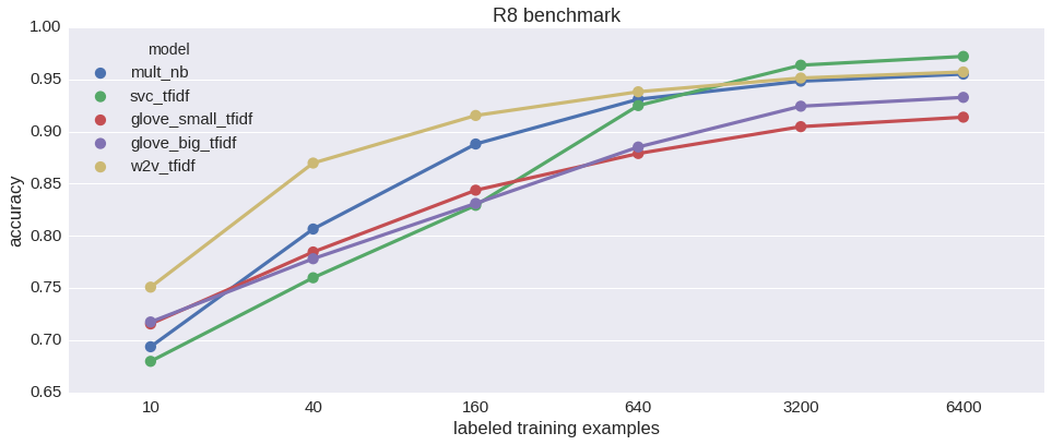
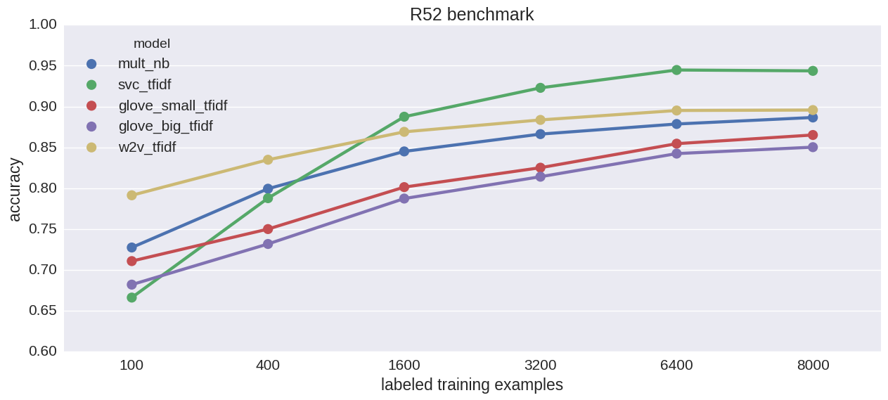
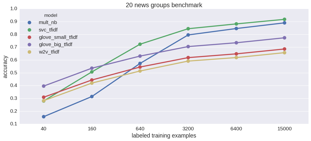
I have blogged about the wide usefulness of topic models and I have benchmarked word-embedding-assisted classification on Reuter’s benchmark. This time I experiment with these ideas using a real world and decent sized dataset - the graph of UK/Irish companies. I have done this during my “10% time” at DueDil (it’s like google’s “20% time”, except it exists).
Graph of companies
There are 4 million active companies in the UK and Ireland. DueDil collects all kinds of information about them - financials, legal structures, contact info, company websites, blogs, news appearences etc. All of it is presented to our users and some of it also serves as input to machine learning tasks - like classifying companies into industries.
One very interesting dataset that remains underutilised (AFAIK by anyone, not just DueDil) is the network of connections of companies and directors.
You can tell a lot about a company just by looking at its directors. That is - if you know anything about these people. At DueDil we don’t know much more than just their identities. This would be rather useless in the context of a single company. But there are millions of companies and people who serve as their directors more often then not do it many times in their careers at different companies. Knowing that the director’s name is Jane Brown may be useless, but knowing that the director previously held similar positions at three different tech startups is highly relevant. And this is just one director out of many and one type of relationship.
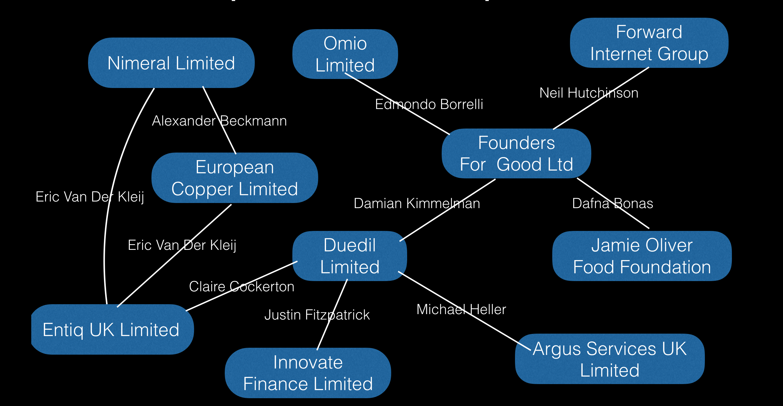
More generally, one can think about companies as nodes in a graph. Two companies are connected iff there is a person who has served as a director at both of them (not necessarily at the same time). I will call this the company graph. Here’s a part of the graph containing DueDil.
DueDil is connected to Founders For Good Ltd because our CEO Damian Kimmelman is also a director at the other company.
It is intuitive that the position of a company in this graph tells us something about the company. It is however difficult to do anything with this information unless it is somehow encoded into numbers.
Company2Vec
This is where word embeddings come in. As I mentioned previously, it is possible to apply Word2Vec to a graph to get an embedding of graph nodes as real-valued vectors in a procedure called DeepWalk. The idea is very simple:
Construct a bunch of random walks on the graph
Feed the random walks into Word2Vec
A random walk is just a sequence of nodes, where the next node is always one of the neighbours of the previous node, chosen at random. Think: Duedil -> Founders For Good Ltd -> Omio Limited.
Word2Vec accepts a collection of documents - where every document is a list of tokens (strings). Here company Id’s play the role of tokens and random walks play the role of documents. It all checks out.
To limit the size of the graph for this proof of concept, I have applied this procedure only to the 2.2 million companies that
are active
have at least one edge (director in common) to another active company
I generated 10 random walks starting at every company, the length of each walk was 40. Training Word2Vec with gensim on this corpus of $10 \times 40 \times 2200000 = 8.8 \times 10^8$ tokens took over 11h. It also took a machine with 40gb of RAM before it stopped crashing even though the random walks were generated on-line.
Finally I got some vectors out of it - one per company. These vectors themselves were the goal of this project (they can serve as features in ML), but I also made some plots to verify that the algorithm is working as advertised.
Pretty pictures with t-SNE and Bokeh
The embedding produced by DeepWalk was 100-dimensional in this case, so I had to do some dimensionality reduction before trying to visualize the vectors. t-SNE is perfect for this kind of thing. Here’s a sample of 40000 company vectors embedded in 2D with t-SNE. You can move or zoom in the plot or hover over the dots to see the names of the corresponding companies.
Bokeh Plot
It worked! You can immediately see that there is some structure in the data and t-SNE has picked up on it (and this is only a tiny sample - 2% of all the datapoints). What does this structure mean? After the graph has beed transformed with DeepWalk and then t-SNE, the position of a company in this plot doesn’t have a simple interpretation but it’s clear that groups of highly interconnected companies will correspond to clusters of points in this plot. And it’s easy to verify just by looking at the names of the companies that this is the case.
Take the big blob in the upper left corner - the companies there:
We have discovered the cluster of irish companies! And if you zoom in on the long, narrow appendage sticking out of this cluster towards bottom left - you’ll see companies like:
Tempelhof Aircraft Leasing (Ireland) Limited
Gallic Dragon Aviation Limited
Aergen Aircraft Ten Limited
… and hundreds more. This is not even cherry-picked. I hereby declare the discoverery of the Irish Aviation Peninsula.
Slightly up and to the right of center there is a smaller scottish cluster recognizable through such companies as
Caledonian Sausage Company
Edinburgh Tattoo Productions Limited
Dundee Ice Arena
There are many other smaller clusters and it’s actually a fun exercise to try to pinpoint exactly what do the companies in a cluster have in common.
Now in color!
This was fun if somewhat grim looking. Let’s try to add some color to the plot. The original goal of this project was to get graph-derived features for industry classification. Let’s try using different colors to denote different industries (based on SIC codes). If DeepWalk coordinates are predictive of the industry a company is in, we should expect to see same-colored dots (companies in the same industry) clustering together in the plot. Does this actually happen?
Bokeh Plot
A little bit, yes.
Mostly everything is a big reddish mess (“services” is the most popular category). But there are indeed some clusters. Right of center we can see a medium sized pink blob of insurance companies:
US Risk (UK) Newco Limited
Zenith Insurance Management UK Limited
North Star Underwriting Limited
Below it and to the left lies another, this one green:
Timeless Films Limited
Hercules Productions Ltd
Koninck studios PTE Limited
Clearly this is a cluster of film companies (plus other media). If you look more closely you will discover that this is actually the cluster of London based film companies. Nearby there is a smaller green cluster of media companies from the rest of England and another one for Wales. These are less clearly delimited and partly obscured by the red dots of “Services” companies. There are many others, but they are sometimes so tight, they appear as a single dot in the plot.
This is more noisy than I hoped for but it’s definitely working. Would definitely improve accuracy of industry classification if used with other stronger features. Plus you can learn interesting things from it just by looking at the plot. Like the fact that film production companies are closely connected to each other and relatively unconnected to the rest of the world. Or that London is a different country as far as media companies are concerned.
Bonus: keyword based company embedding
Having all this t-SNE and Bokeh niceness in place I couldn’t resist applying it to another interesting dataset - keywords. Keywords are a set of industry related tags that DueDil has for millions of companies. They are things like “fishing” or “management consulting” or “b2b”. A company usually has between a few and a few dozen of them.
A byproduct of the pipeline that extracts keywords for companies is a Word2Vec embedding of the keywords. I used this embedding to create an embedding of companies. This was done simply by averaging all the vectors corresponding to a company’s keywords. I ran the resulting vectors through t-SNE and here’s what it looks like:
Bokeh Plot
I shouldn’t be surprised that keywords - which were picked to be industry related - predict the industry really well. But I was blown away by the level of detail preserved by t-SNE. There are recognizable islands for everything. There is a golden Farmers Archipelago and a narrow blue Dentist Island south from Home Care Island. There is a separate Asian Island in the Restaurant Archipelago - go see for yourself.
I will share with you a snippet that took out a lot of misery from my dealing with pyspark dataframes. This is pysparks-specific. Nothing to see here if you’re not a pyspark user. The first two sections consist of me complaining about schemas and the remaining two offer what I think is a neat way of creating a schema from a dict (or a dataframe from an rdd of dicts).
The Good, the Bad and the Ugly of dataframes
Dataframes in pyspark are simultaneously pretty great and kind of completely broken.
they enforce a schema
you can run SQL queries against them
faster than rdd
much smaller than rdd when stored in parquet format
pyspark dataframe outer join acts as an inner join
when cached with df.cache() dataframes sometimes start throwing key not found and Spark driver dies. Other times the task succeeds but the the underlying rdd becomes corrupted (field values switched up).
not really dataframe’s fault but related - parquet is not human readable which sucks - can’t easily inspect your saved dataframes
But the biggest problem is actually transforming the data. It works perfectly on those contrived examples from the tutorials. But I’m not working with flat SQL-table-like datasets. Or if I am, they are already in some SQL database. When I’m using Spark, I’m using it to work with messy multilayered json-like objects. If I had to create a UDF and type out a ginormous schema for every transformation I want to perform on the dataset, I’d be doing nothing else all day, I’m not even joking. UDFs in pyspark are clunky at the best of times but in my typical usecase they are unusable. Take this, relatively tiny record for instance:
And this is what I would have to type every time I need a udf to return such record - which can be many times in a single spark job.
Dataframe from an rdd - how it is
For these reasons (+ legacy json job outputs from hadoop days) I find myself switching back and forth between dataframes and rdds. Read some JSON dataset into an rdd, transform it, join with another, transform some more, convert into a dataframe and save as parquet. Or read some parquet files into a dataframe, convert to rdd, do stuff to it, convert back to dataframe and save as parquet again. This workflow is not so bad - I get the best of both worlds by using rdds and dataframes only for the things they’re good at. How do you go from a dataframe to an rdd of dictionaries? This part is easy:
1
rdd=df.rdd.map(lambdax:x.asDict())
It’s the other direction that is problematic. You would think that rdd’s method toDF() would do the job but no, it’s broken.
1
df=rdd.toDF()
actually returns a dataframe with the following schema (df.printSchema()):
It interpreted the inner dictionary as a map of boolean instead of a struct and silently dropped all the fields in it that are not booleans. But this method is deprecated now anyway. The preferred, official way of creating a dataframe is with an rdd of Row objects. So let’s do that.
In addition to this, both these methods will fail completely when some field’s type cannot be determined because all the values happen to be null in some run of the job.
Also, quite bizarrely in my opinion, order of columns in a dataframe is significant while the order of keys is not. So if you have a pre-existing schema and you try contort an rdd of dicts into that schema, you’re gonna have a bad time.
How it should be
Without further ado, this is how I now create my dataframes:
1234567891011121314
# this is what a typical record in the rdd looks likeprototype={'first_name':'nadbor','last_name':'drozd','occupation':'data scientist','children':[{'name':'Lucja','age':3,'likes cold showers':True}]}df=df_from_rdd(rdd,prototype,sqlContext)
This doesn’t randomly break, doesn’t drop fields and has the right schema. And I didn’t have to type any of this StructType([StructField(... nonsense, just plain python literal that I got by running
1
printrdd.first()
As an added bonus now this prototype is prominently displayed at the top of my job file and I can tell what the output of the job looks like without having to decode parquet files. Self documenting code FTW!
How to get there
And here’s how it’s done. First we need to implement our own schema inference - the way it should work:
12345678910111213141516171819
importpyspark.sql.typesaspstfrompyspark.sqlimportRowdefinfer_schema(rec):"""infers dataframe schema for a record. Assumes every dict is a Struct, not a Map"""ifisinstance(rec,dict):returnpst.StructType([pst.StructField(key,infer_schema(value),True)forkey,valueinsorted(rec.items())])elifisinstance(rec,list):iflen(rec)==0:raiseValueError("can't infer type of an empty list")elem_type=infer_schema(rec[0])foreleminrec:this_type=infer_schema(elem)ifelem_type!=this_type:raiseValueError("can't infer type of a list with inconsistent elem types")returnpst.ArrayType(elem_type)else:returnpst._infer_type(rec)
Using this we can now specify the schema using a regular python object - no more java-esque abominations. But this is not all. We will also need a function that transforms a python dict into a rRw object with the correct schema. You would think that this should be automatic as long as the dict has all the right fields, but no - order of fields in a Row is significant, so we have to do it ourselves.
def_rowify(x,prototype):"""creates a Row object conforming to a schema as specified by a dict"""def_equivalent_types(x,y):iftype(x)in[str,unicode]andtype(y)in[str,unicode]:returnTruereturnisinstance(x,type(y))orisinstance(y,type(x))ifxisNone:returnNoneelifisinstance(prototype,dict):iftype(x)!=dict:raiseValueError("expected dict, got %s instead"%type(x))rowified_dict={}forkey,valinx.items():ifkeynotinprototype:raiseValueError("got unexpected field %s"%key)rowified_dict[key]=_rowify(val,prototype[key])forkeyinprototype:ifkeynotinx:raiseValueError("expected %s field but didn't find it"%key)returnRow(**rowified_dict)elifisinstance(prototype,list):iftype(x)!=list:raiseValueError("expected list, got %s instead"%type(x))return[_rowify(e,prototype[0])foreinx]else:ifnot_equivalent_types(x,prototype):raiseValueError("expected %s, got %s instead"%(type(prototype),type(x)))returnx
And finally:
12345
defdf_from_rdd(rdd,prototype,sql):"""creates a dataframe out of an rdd of dicts, with schema inferred from a prototype record"""schema=infer_schema(prototype)row_rdd=rdd.map(lambdax:_rowify(x,prototype))returnsql.createDataFrame(row_rdd,schema)
In the previous post I talked about usefulness of topic models for non-NLP tasks, it’s back to NLP-land this time. I decided to investigate if word embeddings can help in a classic NLP problem - text categorization. Full code used to generate numbers and plots in this post can be found here: python 2 version and python 3 version by Marcelo Beckmann (thank you!).
Motivation
The basic idea is that semantic vectors (such as the ones provided by Word2Vec) should preserve most of the relevant information about a text while having relatively low dimensionality which allows better machine learning treatment than straight one-hot encoding of words. Another advantage of topic models is that they are unsupervised so they can help when labaled data is scarce. Say you only have one thousand manually classified blog posts but a million unlabeled ones. A high quality topic model can be trained on the full set of one million. If you can use topic modeling-derived features in your classification, you will be benefitting from your entire collection of texts, not just the labeled ones.
Getting the embedding
Ok, word embeddings are awesome, how do we use them? Before we do anything we need to get the vectors. We can download one of the great pre-trained models from GloVe:
or we can train a Word2Vec model from scratch with gensim:
1234
importgensim# let X be a list of tokenized texts (i.e. list of lists of tokens)model=gensim.models.Word2Vec(X,size=100)w2v=dict(zip(model.wv.index2word,model.wv.syn0))
The (python) meat
We got ourselves a dictionary mapping word -> 100-dimensional vector. Now we can use it to build features. The simplest way to do that is by averaging word vectors for all words in a text. We will build a sklearn-compatible transformer that is initialised with a word -> vector dictionary.
12345678910111213141516
classMeanEmbeddingVectorizer(object):def__init__(self,word2vec):self.word2vec=word2vec# if a text is empty we should return a vector of zeros# with the same dimensionality as all the other vectorsself.dim=len(word2vec.itervalues().next())deffit(self,X,y):returnselfdeftransform(self,X):returnnp.array([np.mean([self.word2vec[w]forwinwordsifwinself.word2vec]or[np.zeros(self.dim)],axis=0)forwordsinX])
Let’s throw in a version that uses tf-idf weighting scheme for good measure
1234567891011121314151617181920212223242526
classTfidfEmbeddingVectorizer(object):def__init__(self,word2vec):self.word2vec=word2vecself.word2weight=Noneself.dim=len(word2vec.itervalues().next())deffit(self,X,y):tfidf=TfidfVectorizer(analyzer=lambdax:x)tfidf.fit(X)# if a word was never seen - it must be at least as infrequent# as any of the known words - so the default idf is the max of # known idf'smax_idf=max(tfidf.idf_)self.word2weight=defaultdict(lambda:max_idf,[(w,tfidf.idf_[i])forw,iintfidf.vocabulary_.items()])returnselfdeftransform(self,X):returnnp.array([np.mean([self.word2vec[w]*self.word2weight[w]forwinwordsifwinself.word2vec]or[np.zeros(self.dim)],axis=0)forwordsinX])
These vectorizers can now be used almost the same way as CountVectorizer or TfidfVectorizer from sklearn.feature_extraction.text. Almost - because sklearn vectorizers can also do their own tokenization - a feature which we won’t be using anyway because the benchmarks we will be using come already tokenized. In a real application I wouldn’t trust sklearn with tokenization anyway - rather let spaCy do it.
Now we are ready to define the actual models that will take tokenised text, vectorize and learn to classify the vectors with something fancy like Extra Trees. sklearn’s Pipeline is perfect for this:
I benchmarked the models on everyone’s favorite Reuters-21578 datasets. Extra Trees-based word-embedding-utilising models competed against text classification classics - Naive Bayes and SVM. Full list of contestants:
mult_nb - Multinomial Naive Bayes
bern_nb - Bernoulli Naive Bayes
svc - linear kernel SVM
glove_small - ExtraTrees with 200 trees and vectorizer based on 50-dimensional gloVe embedding trained on 6B tokens
glove_big - same as above but using 300-dimensional gloVe embedding trained on 840B tokens
w2v - same but with using 100-dimensional word2vec embedding trained on the benchmark data itself (using both training and test examples [but not labels!])
Each of these came in two varieties - regular and tf-idf weighted.
The results (on 5-fold cv on a the R8 dataset of 7674 texts labeled with 8 categories):
SVM wins, word2vec-based Extra Trees is a close second, Naive Bayes not far behind. Interestingly, embedding trained on this relatively tiny dataset does significantly better than pretrained GloVe - which is otherwise fantastic. Can we do better? Let’s check how do the models compare depending on the number of labeled training examples. Due to its semi-supervised nature w2v should shine when there is little labeled data.
That indeed seems to be the case. w2v_tfidf’s performance degrades most gracefully of the bunch. SVM takes the biggest hit when examples are few. Lets try the other two benchmarks from Reuters-21578. 52-way classification:
Qualitatively similar results.
And 20-way classification:
This time pretrained embeddings do better than Word2Vec and Naive Bayes does really well, otherwise same as before.
Conclusions
SVM’s are pretty great at text classification tasks
Models based on simple averaging of word-vectors can be surprisingly good too (given how much information is lost in taking the average)
but they only seem to have a clear advantage when there is ridiculously little labeled training data
At this point I have to note that averaging vectors is only the easiest way of leveraging word embeddings in classification but not the only one. You could also try embedding whole documents directly with Doc2Vec. Or use Multinomial Gaussian Naive Bayes on word vectors. I have tried the latter approach but it was too slow to include in the benchmark.
Update 2017: actually, the best way to utilise the pretrained embeddings would probably be this https://blog.keras.io/using-pre-trained-word-embeddings-in-a-keras-model.html I shall add this approach to the benchmark when I have some time.
Sometimes pretrained embeddings give clearly superior results to word2vec trained on the specific benchmark, sometimes it’s the opposite. Not sure what is going on here.
Overall, we won’t be throwing away our SVMs any time soon in favor of word2vec but it has it’s place in text classification. Like when you have a tiny training set or to ensemble it with other models to gain edge in Kaggle.
Plus, can SVM do this:
12345678910
X=[['Berlin','London'],['cow','cat'],['pink','yellow']]y=['capitals','animals','colors']etree_glove_big.fit(X,y)# never before seen words!!!test_X=[['dog'],['red'],['Madrid']]printetree_glove_big.predict(test_X)
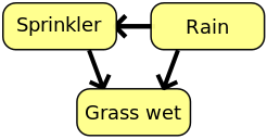
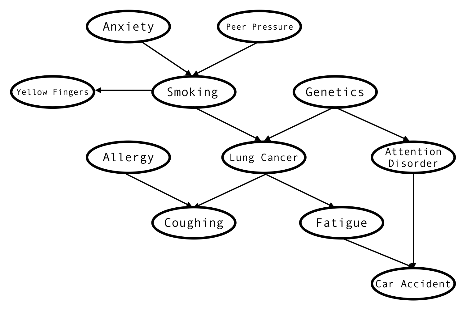
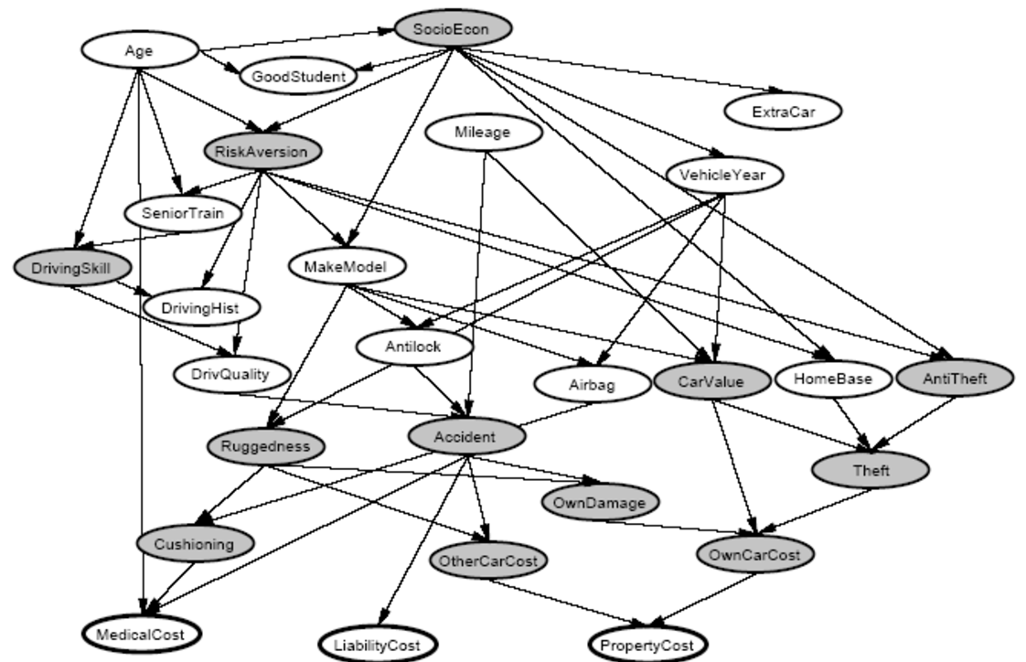
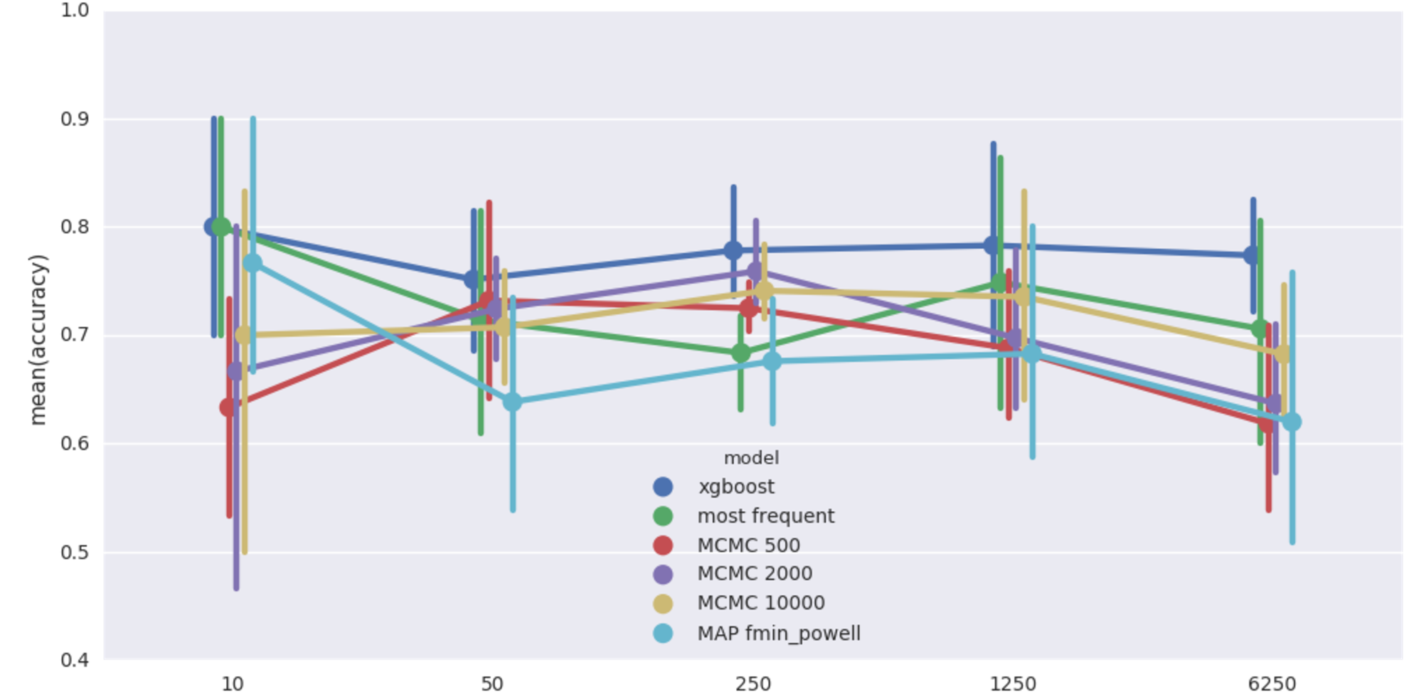 Rain-Sprinkler-Wet Sidewalk benchmark (20% missing values). Mean imputation accuracy from 5 runs vs data size.
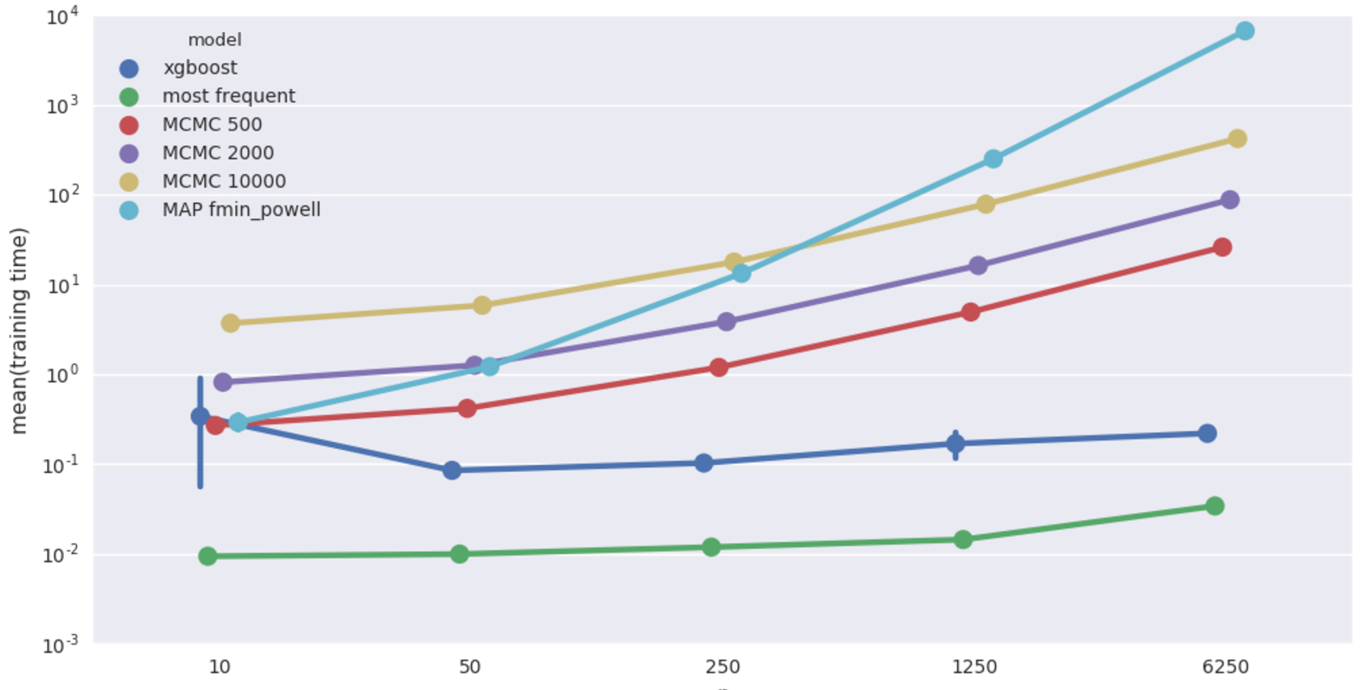 Average fitting time in seconds. Beware log scale!
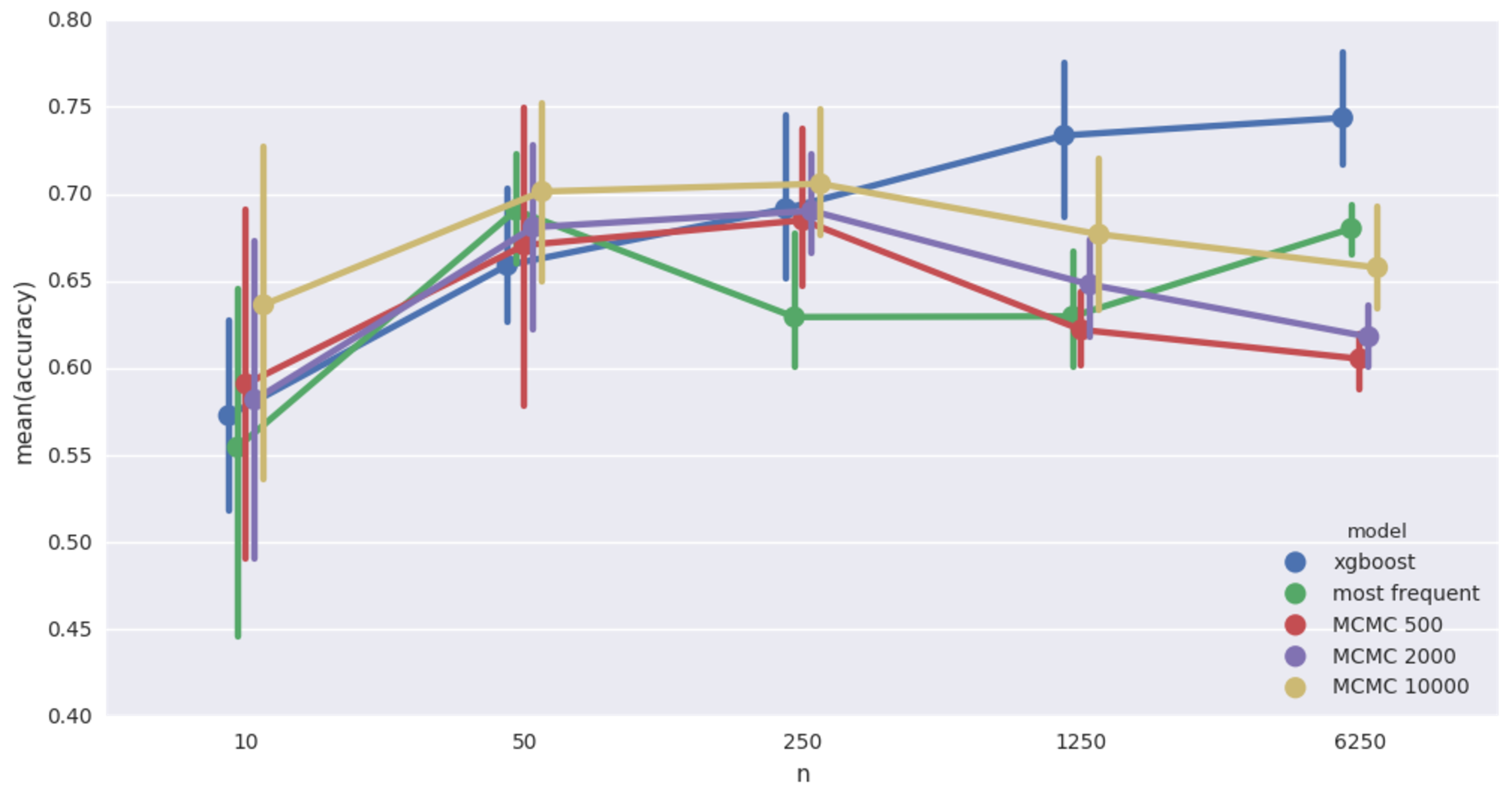 Cancer network imputation accuracy. 20% missing values
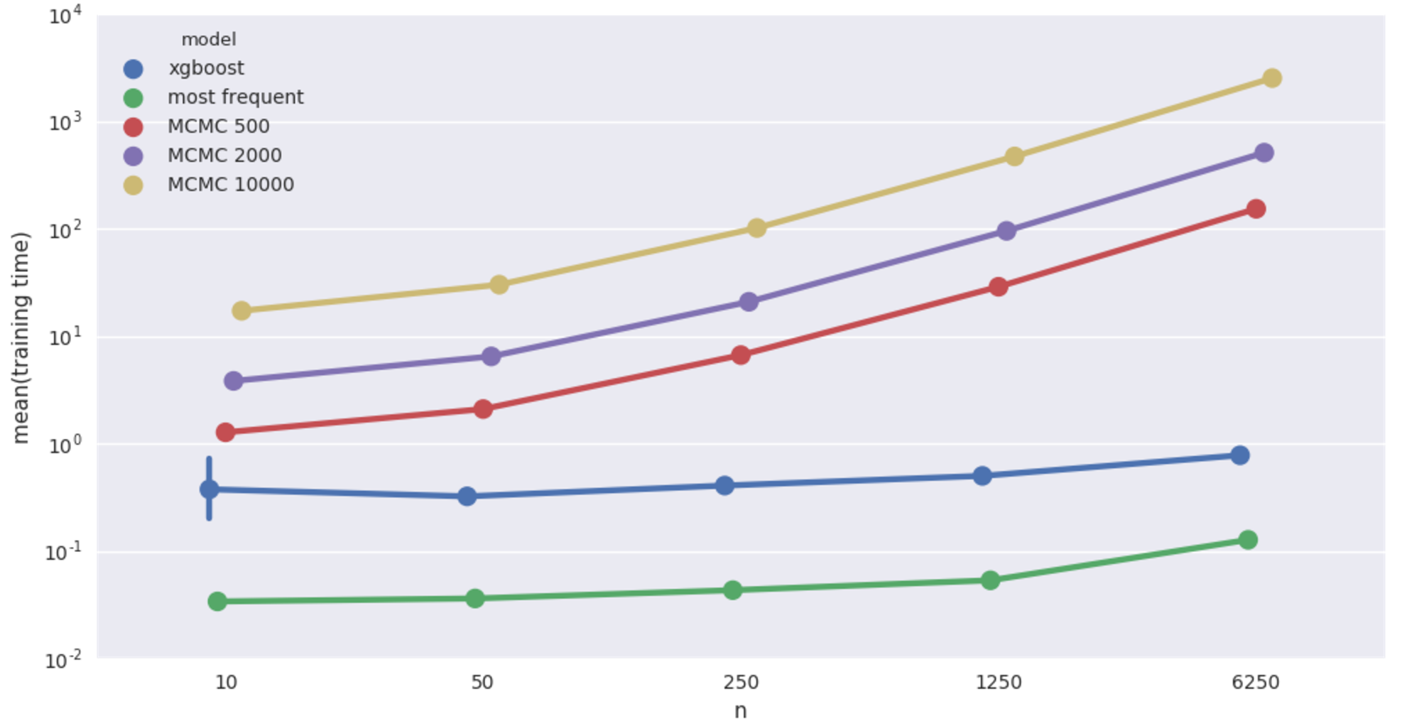 Cancer network imputation time.
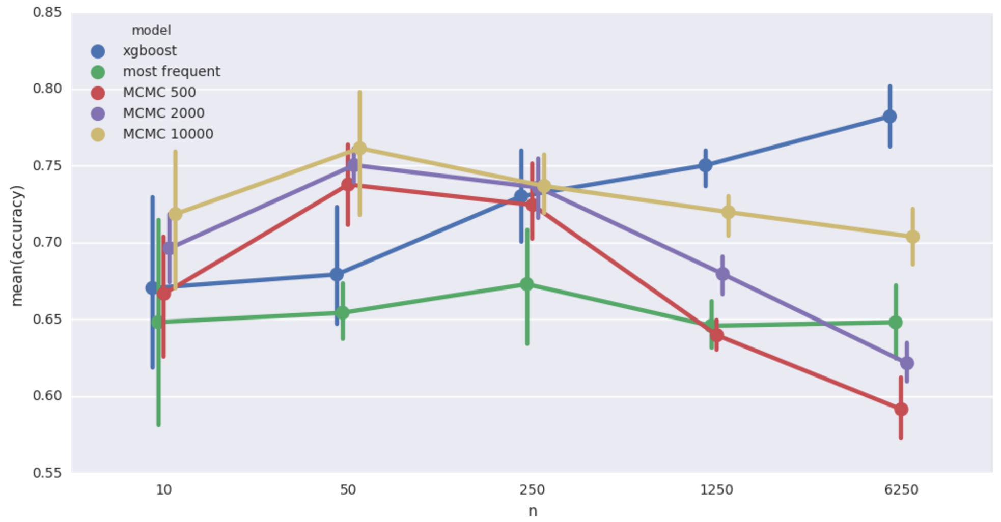 Car insurance network imputation accuracy. 20% missing values
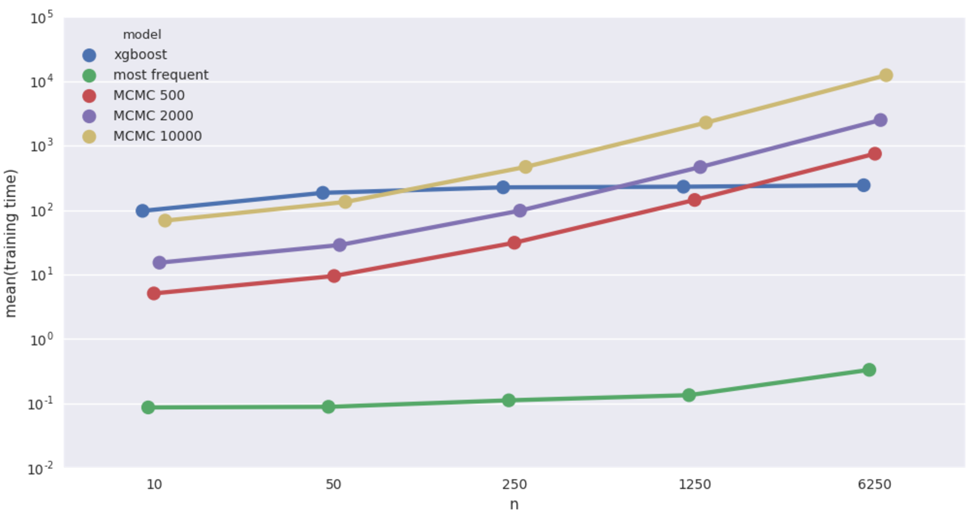 Car insurance network imputation time.
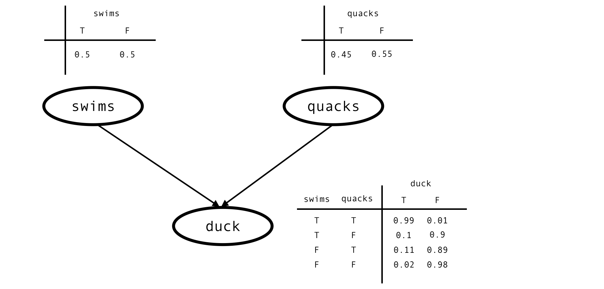
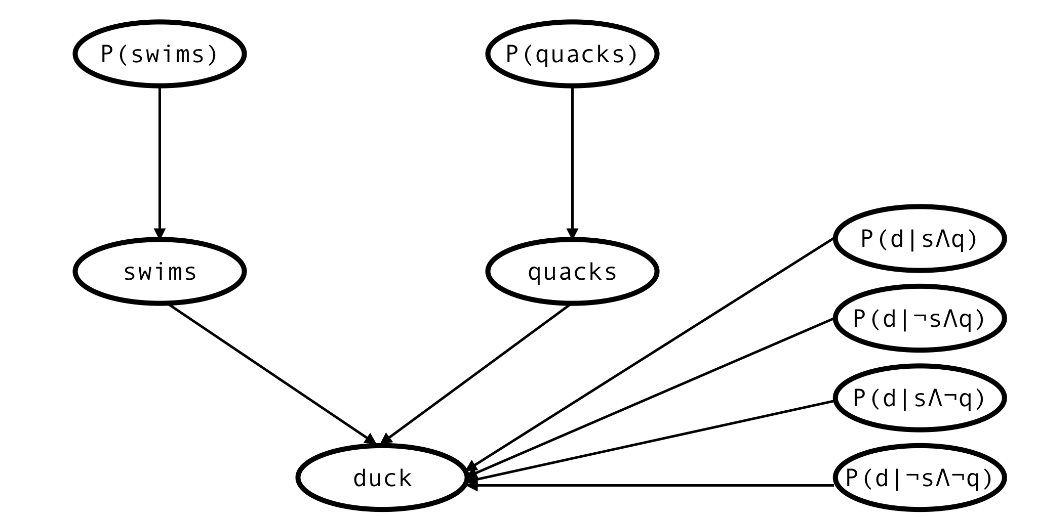
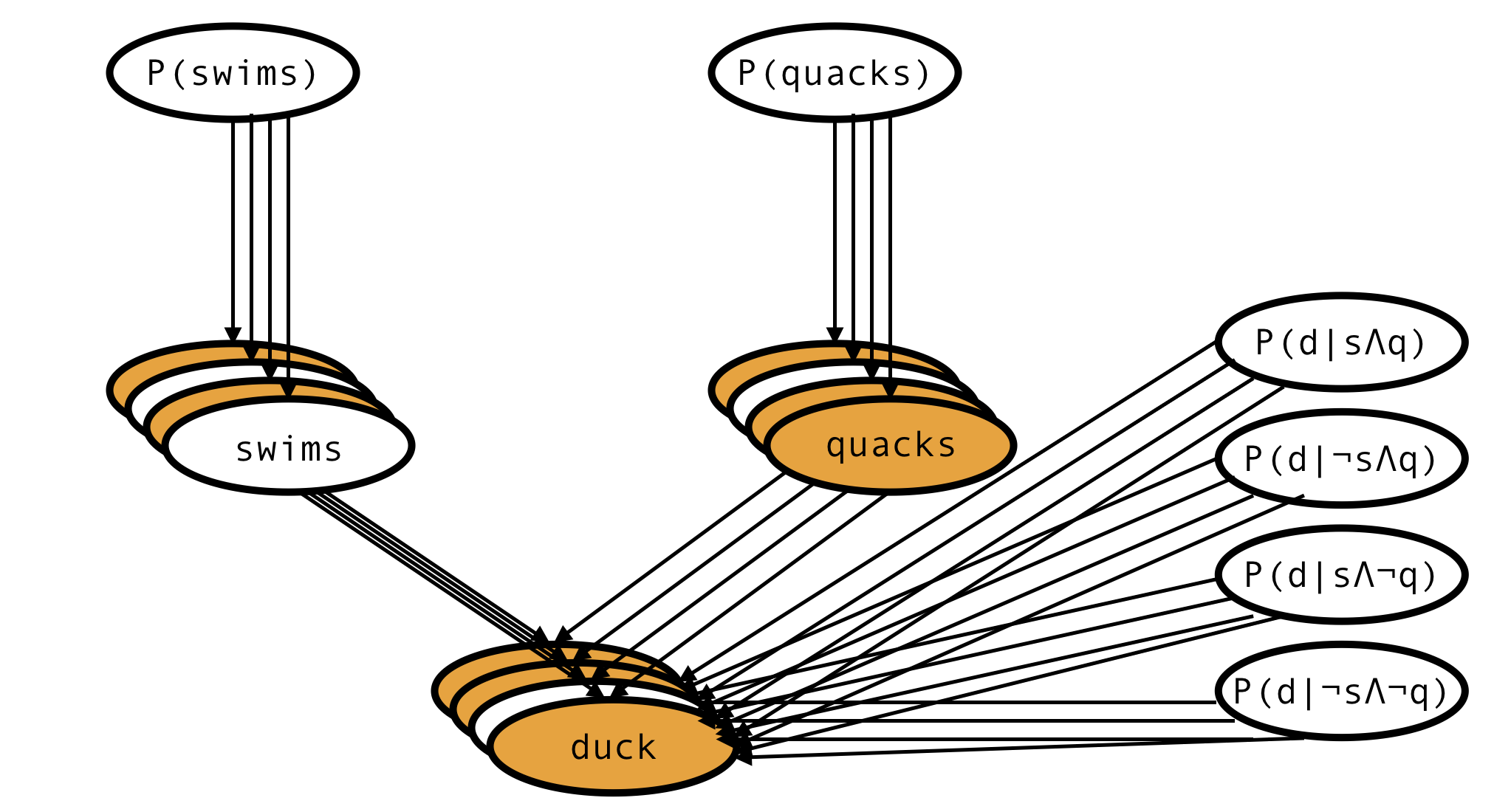
 watercooling, pretty lights and 2 x GTX 1080 (on the right)