This post will be about a cool new feature engineering technique for encoding sets of vectors as a single vector - as described in the recent paper An efficient manifold density estimator for all recommendation systems. The paper focuses on EMDE’s applications to recommender systems but I’m more interested in the technique itself.
I will provide motivation for the technique, a python implementation of it and finally some benchmarks.
Aggregating vectors as feature engineering
From a pragmatic perspective, EMDE is just an algorithm for compressing sets of vectors into a single fixed-width vector.
Aggregating a set of vectors into a single vector may seem like a pretty esoteric requirement but it is actually quite common. It often arises when you have one kind of entities (users) interacting with another (items, merchants, websites).
Let’s say you already have a vector representation (embedding) of every food item in the world. Like any good embedding, it captures the metric relations between the underlying objects - similar foods are represented by similar vectors and vice versa. You also have a list of people and the foods they like. You would like to leverage the food embeddings to create embeddings of the people - for the purpose of recommendation or classification or any other person-based ML task.
Somehow you want to turn the information that Alice likes salami, chorizo and Hawaiian pizza (mapped to vectors v1, v2, v3) into a single vector representing Alice. The procedure should work regardless of how many food items a person likes.
Aggregating vectors as density estimation
Another way of looking at the same problem - and one taken by the authors of the EMDE paper - is as a problem of estimation of a density function in the embedding space.
Instead of thinking of foods as distinct points in space, we can imagine a continuous shape - a manifold - in the embedding space whose every point corresponds to a food - real or potential. Some of the points on this manifold are familiar - an apple or a salami. But between the familiar ones there is a whole continuum of foods that could be. An apple-flavored salami? Apple and salami salad? If prosciutto e melone is a thing, why not salami apple?
In this model we can think of Alice’s preferences as a probability density function defined on the manifold. Maybe function’s value is highest in the cured meats region of the manifold, lower around pizzas and zero near the fruits. That means Alice likes salami, chorizo, pepperoni and every other similar sausage we can invent but she only likes some pizzas and none of the fruits.
This density function is latent - we can’t measure it directly. All we know is the handful of foods that Alice explicitly liked. We can interpret these items as points drawn from the latent probability distribution. What we’re trying to do is use the sample to get an estimate of the pdf. The reason this estimation is at all possible is that we believe the function is well-behaved in the embedding space - it doesn’t vary too wildly between neighbouring items. If Alice likes salami and chorizo, she will also probably like other similar kinds of sausage like pepperoni.
Viewed from this perspective, the purpose of EMDE is to:
Parametrize the space of all probability distributions over the manifold of food items.
Estimate the paramaters of a specific distribution based on a sample.
The estimated parameters can then serve as a feature vector describing the user.
How not to do it
The most straightforward way of summarising a list of vectors is by taking their arithmetic average. That’s exactly what I have tried in my post from 2016. It worked okay-ish as a feature engineering technique but clearly a lot of detail gets lost this way. For instance, by looking at just the average vector, you can’t tell the difference between someone who likes hot dogs and someone else who only likes buns and frankfurters separately.
The average is just a summary statistic of a distribution - but what EMDE is trying to do is capture the full distribution itself (up to a finite but arbitrary precision).
EMDE - idea
The input to this algorithm consists of:
the set of embeddings of all items
list of items per user
And the hyperparameters:
K - the number of hyperplanes in a single partitioning
and N - the number of independent partitionings
The output is a sparse embedding of each user.
The algorithm (the illustrations will use K=3 and N=4):
1.
Start with the set of embeddings of all items.
2.
Cut the space into regions (buckets) using random hyperplanes. The orientation of the hyperplanes is uniformly random and their position is drawn from the distribution of the item vectors. That means the planes always cut through the data and most often through regions where data is dense, never outside the range of data.
Assign numbers to the regions.
3.
For each user count items in each bucket.
The sequence of numbers generated this way
1
[0, 0, 2, 0, 0, 0, 1]
is the desired summary of the user’s items (almost). It is easy to see that these numbers define a coarse-grained density function over the space of items - like so:
4.
To get a more fine-grained estimate of the latent density, we need to repeat steps 2. and 3. N times and concatenate the resulting count vectors per user.
This sequence of numbers (the authors of the paper call it a “sketch” as it is a kind of a Count Sketch)
is the final output of EMDE (for one particular user).
The corresponding density function would look something like this:
Two important properties of this algorithm:
The resulting sketches are additive - sketch({apple, salami}) = sketch({apple}) + sketch({salami}).
Similar items tend to fall into the same bucket so they end up with a similar sketch - sketch({apple, salami}) ~ sketch({pear, chorizo}).
K and N
The authors of the EMDE paper suggest that sketch width = 128 (roughly corresponding to K=7) is a good default setting and one should spend one’s dimensionality budget on increasing N rather than K beyond this point.
But why bother with N sets of hyperplanes at all? Why not use all of them in one go (N=1, big K)?
The answer (I think) is that we don’t want the buckets to get too small. The entire point of EMDE is to have multiple similar items land in the same bucket - otherwise it’s just one-hot encoding. OHE is not a bad thing in itself but it’s not leveraging the embeddings anymore.
Having large buckets (small K), on the other hand leads to false positives - dissimilar items landing in the same bucket - but we mitigate this problem by having N overlapping sets of buckets. Even if bananas and chorizo end up in the same bucket one of the sets, they probably won’t in the others.
That being said, I have tried lots of different combinations of K and N and can’t see any clear pattern regarding what works best.
EMDE - implementation
Once trained on a set of vectors, EMDE can be used to transform any other sets of vectors - as long as they have the same dimension. However, in most applications, all the item vectors are static and known up front. The following implementation will assume that this is the case which will let us make the code cleaner and more efficient. I have included the more general, less efficient implementation here.
Thanks to additivity of sketches, to find the sketch of any given set of items it is enough to find the sketches of all the individual items and add them. Since all the items are know at training time, we can just pre-calculate sketches for all of them and simply add them at prediction time.
The following function pre-calculates sketches for all the items given their embeddings.
Linear algebra 101 reminder: a hyperplane is the set of points $\vec{x}$ in a Euclidean space that satisfy:
for some constant $\vec{v}$, $c$.
If $\vec{v} \cdot \vec{x} > c$ - then $\vec{x}$ lies to one side of the hyperplane. If $\vec{v} \cdot \vec{x} < c$ - it lies on the other side.
importnumpyasnpfromsklearn.feature_extraction.textimportCountVectorizerimportscipy.sparseassspdefEMDE_transform(K,N,item_vectors):"""takes a and array of embedding vectors and returns a sparse array of their sketches """n_items,d=item_vectors.shapeshallow_sketches=[]for_inrange(N):# first chose K vectors at random - these are the normal vectors to the K hyperplanesrandom_vectors=np.random.normal(size=(K,d))# for every hyperplane choose one of the items at random# we will choose the offset for the hyperplane so that it passes# through the selected item (or rather the item's vector)random_inds=np.random.randint(n_items,size=K)# scalar product of every item with the random vectorsscalar_products=random_vectors.dot(item_vectors.T)offsets=scalar_products[range(K),random_inds]# for every point for every plane determine # on which side of the plane does the point lie# the result is a boolean array of size (n_items, K)bits=(scalar_products>offsets.reshape([K,1])).T# for every item encode the sequence of booleans as an integer using binary# the result is an integer array of length n_itemsbucket_nums=(bits*(2**np.arange(K))).sum(axis=1)# one-hot-encoding on bucket numberssketch=CountVectorizer(analyzer=lambdax:x).fit_transform(bucket_nums.reshape(n_items,1))shallow_sketches.append(sketch)returnssp.hstack(shallow_sketches)
Note that CountVectorizer above makes sure that only the buckets with at least one vector in them are represented. As a result, the width of a single sketch which is at most $2^K$ ($2^K N$ for the full sketch), in practice is often much lower - especially for low dimensional embeddings.
Now, for convenience, we can wrap this up in a sklearn-like interface while adding the option to use tfidf weighting for items.
1234567891011121314151617181920
classEMDEVectorizer(object):"""A drop-in replacement for CountVectorizer and TfidfVectorizer - based on EMDE"""def__init__(self,K,N,item2vec,tfidf=False):items=list(item2vec.keys())item_vectors=np.vstack(list(item2vec.values()))self.emde_embeddings=EMDE_transform(K,N,item_vectors)iftfidf:self.vectorizer=TfidfVectorizer(analyzer=lambdax:x,vocabulary=items)else:self.vectorizer=CountVectorizer(analyzer=lambdax:x,vocabulary=items)deffit(self,X,y=None):# this is only necessary for tfidf=True, otherwise it does nothingself.vectorizer.fit(X)returnselfdeftransform(self,X):returnself.vectorizer.transform(X).dot(self.emde_embeddings)
Before passing this sketch to a ML model, you might want to normalize it row-wise. The paper suggests ‘L2’ normalization. I’ve had even better results with max norm:
In both cases I trained Word2Vec on all the texts to get a word embedding and then used EMDE to generate a sketch for every document by aggregating the word embeddings. Then I trained and tested a logistic regression (with 5-fold cross validation) on the sketches as well as on the raw word counts and on averaged embeddings.
First of all - you’ll notice that all the EMDE dimensionalities tend to be lower for the R8 dataset than for 20 Newsgroups. That is because R8 is a much smaller dataset with fewer distinct words in it (23k vs 93k). Consequently you more often end up with an empty bucket - and those get dropped by CountVectorizer.
As for the actual results:
overall (some) EMDE sketches beat one-hot-encoding on both benchmarks and by a fairly wide margin
averaging embedding vectors doesn’t perform well at all
the higher dimensional sketches tend to do better on these datasets
there is no clear pattern regarding the importance of increasing K vs N. K=30 N=1 is on top of one of the benchmarks. K=30 N=2000 wins in the other
In conclusion - EMDE is simple, fast, efficient. It will make a great addition to the feature engineering arsenal of any data scientist.
In this post I explain why graph embedding is cool, why Pytorch BigGraph is a cool way to do it and show how to use PBG on two very simple examples - the “Hello World!” of graph embedding.
All the code can be found here. With this you can quickly get started embedding your own graphs.
Example: Graph of movies
Before we get started, here’s a motivating example: visualisation of the Movies Dataset from Kaggle.
The above embedding was based on a multi-relation graph of people working on movies (actors, directors, screenwriters, lightning, cameras etc.). The visualisation is the result of running UMAP on the embeddings of the most popular movies (ignoring embeddings of people which were a by-product).
And here’s the same set of movies but with a different embedding:
This embedding was based on the graph of movie ratings. The nodes correspond to movies and raters. There are 3 types of edges - ‘this user hated this movie’, ‘this user found this movie acceptable’, ‘this user loved this movie’ - corresponding to ratings 1 to 2.5, 3 to 3.5, 4 to 5 out of 5.
I encourage you to mouse over the graphs to reveal clusters of movies related by either overlapping cast and crew (first plot) or by overlapping fanbase (second plot). It’s quite fun.
Note that one could use either of these embeddings (or a combination of the two) as a basis for a movie recommender system.
Why graph embeddings?
Graph embeddings are a set of algorithms that given a graph (set of nodes connected by edges) produce a mapping node -> n-dimensional vector (for some specified n). The goal of embedding is for the metric relationships between vectors to reflect connections of the graph. If two nodes are connected, their embeddings should be close in vector space (under some metric), if they are not - the embeddings should be distant.
If successful, the embedding encodes much of the structure of the original graph but in a fixed-width, dense numeric format that can be directly used by most machine learning models.
Unlike their better known cousins - word embeddings - graph embeddings are still somewhat obscure and underutilised in the data science community. That must be in part because people don’t realise that graphs are everywhere.
Most obviously, when the entities you’re studying directly interact with each other - they form a graph. Think - people following each other on social media or bank customers sending each other money.
More common in real life applications are bipartite graphs. That’s when there are two kinds of entities - A and B - and As link with Bs but As don’t link with other As directly and neither do Bs with other Bs. Think - shoppers and items, movies and reviewers, companies and directors. Embedding these kinds of graphs is a popular technique in recommender systems - see for example Uber Eats.
Text corpora are graphs too! You can represent each document in a corpus and each word in a document by a node. Then you connect a document-node to a word-node if the document contains the word. That’s your graph. Embedding this graph yields a word embedding + document embedding for free. (you can also use a sliding window of a few words instead of full document for better results). This way you can get a good quality word embedding using graph embedding techniques (see e.g. this).
In short - graph embeddings are a powerful and universal feature engineering technique that turns many kinds of sparse, unstructured data into dense, structured data for use in downstream machine learning applications.
Why PyTorch BigGraph
There are heaps of graph embedding algorithms to pick from. Here’s a list of models with (mostly Python) implementations. Unfortunately most of them are little better than some researcher’s one-off scripts. I think of them less as tools that you can pick up and use and more as a starting point to building your own graph embedder.
PyTorch BigGraph is by far the most mature of the libraries I have seen. It:
includes utils for transforming edge-list data to it’s preferred format.
includes multiple metrics for monitoring performance during as well as after training
supports multi-relation and multi-entity graphs
is customizable enough that it supersedes multiple other older models
is CPU-based - which is unusual and seems like a wasted opportunity but it does make using it easier and cheaper
And most importantly:
it is fast and works reliably on even very big graphs (being disk-based, it won’t run out of RAM)
It even includes a distributed mode for parallelizing training on the cluster. Unless the nodes of your graph number in the billions though, IMHO it is easier to just spin up a bigger machine at your favourite cloud platform. In my experiments a 16 CPU instance is enough to embed a graph of 25m nodes, 30m edges in 100d in a few hours.
If you’re curious about
Why this tutorial?
If PBG is so great why does it need a tutorial?
It seems to me that the authors were so focused on customizability that they let user experience take a back seat. Simply put - it takes way too many lines of code to do the simplest thing in PBG. The simplest usage example included in the repository consists of two files - one 108 and one 46 lines long. This is what it takes to do the equivalent of model.fit(data).predict(data).
I’m guessing this is the reason why the library hasn’t achieved wider adoption. And without a wide user base, who is there to demand a friendlier API?
I have wasted a lot of time before I managed to refactor the example to work on my graph. What follows is my stripped down to basics version of graph embedding that should work out of the box - the “Hello World!” - and one that you can use as a template for more complicated tasks.
I found another similar tutorial on Towards Data Science but the code didn’t work for me (newer version of PBG perhaps?).
Hello World!
The full code of the example, with comments, is here.
First thing to do is installing PBG. As of this writing, the version available on PyPi is broken (crashes on running the first example) and you have to install it directly from github:
The graph we will be embedding consists of 4 nodes - A, B, C, D and 5 edges between them. It needs to be saved as a tab-separated file like so:
12345
ABBCCDDBBD
Before we can apply PBG to the graph, we will have to transform it to a PBG-friendly format (fortunately P BG provides a function for that). Before we do that, we have to define the training config. The config is a data structure holding all the settings and hyperparameters - like how many partitions to use (1 unless you want to do distributed training), what types of nodes there are (only 1 type), what types of edges between them etc.
raw_config=dict(# graph metadata will go hereentity_path=DATA_DIR,edge_paths=[# graph data in HDF5 format will be saved hereDATA_DIR+'/edges_partitioned',],# trained embeddings as well as temporary files go herecheckpoint_path=MODEL_DIR,# Graph structureentities={"WHATEVER":{"num_partitions":1}},relations=[{"name":"doesnt_matter","lhs":"WHATEVER","rhs":"WHATEVER","operator":"complex_diagonal",}],dynamic_relations=False,dimension=4,# silly graph, silly dimensionalityglobal_emb=False,comparator="dot",num_epochs=7,num_uniform_negs=50,loss_fn="softmax",lr=0.1,regularization_coef=1e-3,eval_fraction=0.,)
Next, we use the config to transform the data into the preferred format using a helper function from torchbiggraph.converters.importers.convert_input_data function. Note that the config needs to be parsed first using another helper function because nothing is simple with PyTorch BigGraph.
12345678910111213141516
setup_logging()config=parse_config(raw_config)subprocess_init=SubprocessInitializer()# path to the tsv file with the graph edgesinput_edge_paths=[Path(GRAPH_PATH)]convert_input_data(config.entities,config.relations,config.entity_path,config.edge_paths,input_edge_paths,TSVEdgelistReader(lhs_col=0,rel_col=None,rhs_col=1),dynamic_relations=config.dynamic_relations,)
Having prepared the data, training is straightforward:
1
train(config,subprocess_init=subprocess_init)
Important note: the above code (both data preparation and training) can’t be at the top level of a module - it needs to be placed inside a if __name__ == '__main__': block or some equivalent. This is because PTBG spawns multiple processes that import this very module at the same time. If this code is at the top level of a module, multiple processes will be trying to create the same file simultaneously and you will have a bad time!
After training is done, we can load the embeddings from a h5 file. This file doesn’t include names of the nodes so we will have to look those up in one of the files created by the preprocessing function.
The second example will feature PBG’s big selling point - the support for multi-relation graphs.
That means graphs with multiple kinds of edges. We will also throw in multiple entity types for good measure.
Imagine if Twitter and eBay had a baby. Data genereated on this unholy abomination of a website might look something like this:
Here users follow other users as well as buy and sell items to each other. As a result we have two types of entities - users and items - and four types of edges - ‘bought’, ‘sold’, ‘follows’ and ‘hates’.
We want to jointly embed users and items in a way that implicitly encodes who is buying and selling what and following or hating whom.
We could do it by ignoring relation types and embedding it as a generic graph. That would be wrong because ‘follows’ and ‘hates’ mean something quite different and we don’t want to represent Bob and Dave as similar just because one of them follows Carol and the other hates her.
Or we could do it by separately embedding 4 graphs - one for each type of relation. But that’s not ideal either because we’re losing valuable information. In our silly example Alice would only appear in the graphs of “bought” and of “follows”. Dave only appears in graphs of “sold” and “hates”. Therefore the two users wouldn’t have a common embedding and it wouldn’t be possible to calculate distance between them. A classfier trained on Alice couldn’t be applied to Dave.
We can solve this problem by embedding the full multi-relation graph in one go in PBG.
Internally, PBG deals with different relation types by applying a different (learned) transaformation to a node’s embedding in the context of a different relation type. For example it could learn that that if A ‘follows’ B, they should be close in vector space but when A ‘hates’ B, they should by close after flipping the sign of all coordinates of A - i.e. they should be represented by opposite vectors.
From the point of view of a PBG user the only difference when embedding a multi-relation, multi-entity graph is that one has to declare all relation types and entity types in the config. We also get to chose a different transformation for each relation (though I can’t imagine why anyone would). The config dict for our Twitter/eBay graph would look like this:
Once embedding is trained, the embeddings can be loaded the same way as with a generic graph, the only difference being that each entity type has a separate embedding file.
I recently came across several articles about failing data science projects (according to Gartner 85% big data projects are never fully productionised). The articles blame misaligned objectives, management resistance, unrealistic expectations, poor communication with stakeholders, poor data infrastructure. I think this is basically correct but too diplomatic. Here’s what I think:
The typical data science project doesn’t make any sense whatsoever and should never have been attempted.
Data science has a huge solution-looking-for-a-problem situation going on. Enterprise managers trying to appear data-driven, startup founders wanting to impress investors with cool buzzwords and proprietary IP, young data scientists themselves itching to try the newest technique from a paper - there are a lot of people looking for an excuse to do ML/AI/DL. When they finally find it, they (or rather - we) don’t try too hard to see if it makes business sense. As a result, the majority of data science projects never move beyond the stage of slides and jupyter notebooks.
Here is my subjective, non-exhaustive list of types of nonsense data science:
1. Vanity data science
By far the most common failure mode for a data science project is to never be productionised because of lack of infrastructure or lack of interest on the business side. These projects were only attempted because thought they sounded cool, in the complete absence of a realistic business case. This could have been avoided by asking a simple question before starting the project:
‘And then what?’
So you apply your DBSCAN on top of your vectors from Word2Vec to assign your customers to clusters - and then what?
Or you run sentiment analysis on all the comments on your website - and then what?
Or you train a GAN on all the images in your database - and then what?
‘How do we productionise the result? Do we have the infrastructure for it? What will the benefit be if we manage to do it?’
If the only answer is ‘and then we prepare slides to show to stakeholders’ - I suggest that we skip the ‘train the neural network’ bit and prepare the slides already. In the unlikely event that the stakeholders have a real use case for the classifier, we can start working on the use case immediately. Otherwise we move on to the next task having saved ourselves weeks, maybe months of unnecessary work.
2. Busywork
Another, less blatant way for a data science project to not make sense is for it to be sort of useful but completely not worth the effort. Like training a bespoke deep learning model to analyse 20 pages of text. Or an image quality assessment tool that saves a real estate agent 5 seconds per 1h house visit.
The question I ask stakeholders (sometimes that means asking myself) to address this problem is:
‘How much is the solution to this problem worth to you? If it’s so valuable, why haven’t you paid people to do it manually before?’
The set of good answers to this question includes:
we have been doing it manually, automating it would save us £X/year
and
we could do it manually but being able to do it in real time would be a game-changer, worth £X.
3. Reinventing the wheel
A special subcategory of ‘obviously not worth it’ projects contains ones where a solution already exists in a commoditised form on AWS, GCP, Azure etc. Examples include OCR, speech to text, generic text and image classification, object detection, named entity recognition and more.
Trying to build (for instance) a better or cheaper OCR than the one Google is selling is first of all hopeless but more importantly a distraction from your actual business (unless you’re business is selling OCR, in which case good luck!).
I sometimes hear data scientists complaining that it’s no fun calling APIs for everything and they would rather build ML models themselves. I disagree. For one, I find solving an already solved problem depressing. Secondly, outsourcing the most generic ML tasks frees up your time to do higher-level tasks and tasks specific to your business. If you really have nothing to do in your company except for reinventing the wheel then you’re in the wrong company.
4. Wishful thinking
The flipside of Busywork Data Science is Wishful Thinking Data Science. Attacking problems that it would be fantastic to have solved but which are obviously not solvable with the given data.
I most often see this kind of thing with predicting the future (which is the hardest period to predict).
Wouldn’t it be great to know the house price index/traffic on the website/demand for a product a year in advance? Can you fit your neural network/hidden markov model to the chart with historical data to make a forecast?
I can fit anything to anything but that won’t tell you much a hand-drawn trend line wouldn’t reveal. Next year’s house prices depend on a million different external political, economic and demographic factors that are either unpredictable or not predictable from price data alone. How the Prime Minister is going to handle Brexit is simply not something that can be divined from squiggly line of past house prices.
Sometimes projects like these are pitched by naive managers and CEOs who think AI is a magic dust you can sprinkle over a problem and make the impossible possible. More often it involves people who either know the prediction won’t work or don’t care enough to find out, their only concern being whether the technology will impress the customer.
5. If you don’t know where you’re going, any road will take you there
This is when the client has a vaguely data-sciencey task but adamantly refuses to specify the objective or acceptance criteria.
- We need you to calculate a score for every company.
- Ok. What do you what this score to measure or predict?
- Dunno. Like, how good they are?
- Good in what way? Good to work at? Good to invest in? A credit rating maybe?
- No, nothing mundane like that.
- Then what?
- You’re the data scientist, we were hoping you would tell us.
- …
- Be sure to include Twitter data!
It’s a normal part of a data scientist’s job to act as a psychoanalyst helping the client discover and articulate what they actually want. But sometimes there is just nothing there to discover because the whole project is just an empty marketing gimmick or an exercise in bureaucratic box-checking.
Conclusion
In 1985 sci-fi comedy movie Weird Science a pair of teenagers make a simulation of a perfect woman on their home computer. After they hook the computer to a plastic doll and hack into a government system, a power surge causes the magical dream woman to come to life.
Today even small children and the elderly are familiar enough with computers to know they don’t work like that. But replace the government system with the cloud, throw in some deep learning references and you’ve got yourself a plausible 2019 movie premise.
Bullshit data science happens because decision makers have the level of understanding of and attitude towards data science the 1980s audiences had for computers. They have unrealistic expectations, are easily bamboozled by it, don’t know how to use it and don’t trust it enough to use where it would make a real difference.
This will eventually change the same way it did with computers in general. The current generation of data scientists will start graduating into management roles, founding their own startups, eventually retiring - same as happened with the programmers from the 1980s.
Until then, we are going to have to fight the bullshit however we can. For data scientists themselves that entails paying more attention to the ‘why’ of what they’re doing, not just the ‘how’. And for the clients the first step would be to involve an experienced and business savvy data scientist from the get go, to help shape what needs to be done instead of just carrying out (potentially nonsensical) orders.
This is the second of a series of posts about things I wish someone had told me when I was first considering a career in data science. Part 1.
For the purposes of this post I define a data analyst as someone who uses tools like Excel and SQL to interrogate data to produce reports, plots, recommendations but crucially doesn’t deliver code. If you work in online retail and create an algorithm recommending tiaras for pets - I call you a data scientist. If you query a database and discover that chihuahua owners prefer pink tiaras and share this finding with the advertising team - you are a data analyst.
Let me get one thing out of the way first: this post is not bashing analysts. Of course data analyst’s work is useful and rewarding in its own right. And there is more demand for it (under various names) than there is for data science. But that is beside the point. The point is that a lot of people will tell you that taking a job as a data analyst is a good way to prepare for data science and that is a lie. In terms of transferable skills you may as well be working as a dentist.
Misconception 1: you can take a job as a data analyst and evolve it into data science as you become more experienced
A data analyst is not a larval stage of a data scientist. They are completely different species.
Data Analyst
Data Scientist
Sits with the business
Sits with engineers (but talks to the business)
Produces reports, presentations
Produces software
Interestingly, the part about sitting in a different place (often a different floor or a different building!) is the bigger obstacle to moving into data science. Independent of having or not having the right skills, a data analyst can’t just up and start doing data science because they don’t have the physical means to do it! They don’t have:
access to full production data
access to tools to do something with that data (hadoop, spark, compute instances)
access to code repositories
While those things can be eventually gotten hold of with enough perseverance, there are other deficits that even harder to make up for:
lack of familiarity with the company’s technological stack
lack of mandate to make necessary changes to that stack/implement features etc.
This should be obvious to anyone who has ever worked in a big company. You don’t simply walk into an software team and start making changes. It sometimes takes months of training for a new developer on the team make first real contribution. For an outsider from a different business unit to do it remotely is unheard of.
Misconception 2: data analysis is good training for data science
you will not be learning about modern machine learning/statistical techniques either - because they are optimised for accuracy and efficiency, not interpretability (which is the analyst’s concern)
You will on the other hand do:
exploratory data analysis
excel, SQL, maybe some one-off R and python scripts
So that doesn’t sound all bad, right? Wrong.
I think a case can be made that the little technical work a data analysts do actually does more harm than good to their data science education. A data scientist and an analyst may be using some of the same tools, but what they do with them is very, very different.
Data analyst’s code
Data Scientist's code
Manually operated sequence of scripts, clicking through GUIs etc.
Fully automated pipelines
Code that only you will ever see
Code that will be used and maintained by other people
One-off, throwaway scripts
Code that is a part of an live app or a scheduled pipeline
Code tweaked until it runs this one time
Code optimised for performance, maintainability and reusability
Doing things a certain way may make sense from a data analyst’s perspective, but the needs of data science are different. When former analysts are thrown into data science projects and start applying the patterns they have developed through the years, the results are not pretty.
Horror story time
Let me illustrate with an example which I promise is not cherry-picked and a fairly typical in my experience.
I joined a project led by analysts-turned-data scientists. We were building prototype of a pipeline doing some machine learning on the client’s data and displaying pretty plots. One of my first questions when I joined was: how are you getting your data from the client? (we needed a new batch of data at that time). The answer was:
Email X in Sweden with a query that he runs on the client’s database. X downloads a csv with results and puts it on an ftp server.
Download the csv from ftp to your laptop.
Upload it to the server where we have Python.
Run a python script on the server to clean the data (the script is in Y’s home directory).
Download the results on your laptop.
Upload results to our database through a GUI.
Run a SQL script in the GUI to join with our other tables (you will find the script in an attachement to some old email).
Download the results.
Upload to our dev MySQL database.
Run another SQL (Y has the script on her laptop).
Pull the data from MySQL into RStudio on the server.
Do actual analytics on the server in R (all of it consists of a single gigantic R script).
Needless to say, this workflow made it impossible to get anything done whatsoever. To even run the pipeline again on fresher data would take weeks (when it should be seconds) and the results were junk anyway because the technologies they used forced them to only use 1% of available data.
On top of that, every single script in the pipeline was extremely hacky and brittle - and here’s why:
When faced with a task, an analyst would start writing code. If it doesn’t work at first, they add to it and tweak it until it does. As soon as a result is produced (a csv file usually), they move on to the next step. No effort is made to ensure reproducibility, reusability, maintainability, scalability. The piece of code gets you from A to B and that is that. A script made this way is full of hard-coded database passwords, paths to local directories, magic constants and untested assumptions about the input data. It resembles a late-game Jenga tower - weird and misshapen, with many blocks missing and others sticking out in weird directions. It is standing for now but you know that it will come crashing down if you as much as touch it.
The tragic part is that none of the people involved in this mess were dumb. No, they were smart and experienced, just not the right kind of experienced. This spaghetti of manual steps, hacky scripts and big data on old laptops is not the result of not enough cleverness. Way too much cleverness if anything. It’s the result of intelligent people with no experience in making software realising too late that they’re out of their depth.
If only my colleagues were completely non-technical - never having written a SAS or SQL script in their lives - they would have had to hire an engineer to do the coding and they themselves would have focused on preparing the spec. This kind of arrangement is not ideal but I guarantee that the result would have been much better. This is why I believe that the data analyst’s experience is not just useless but actively harmful to data science.
Ultimately though the fault doesn’t lie with the analysts but with the management for mismatching people and tasks. It’s time managers understood that:
Data science is software engineering
Software engineering is hard
Software engineering community has developed tools and practices to make it less hard
You need a software professional to wield those tools
Having written a script in SAS doesn’t make one a software professional
Closing remarks
In case I wasn’t clear about this: I am emphatically not saying that analysts can’t learn proper software engineering and data science. If miners can do it, so can analysts. It’s just that an analyst’s experience makes it harder for them (and their managers!) to realise that they are missing something and easier to get by without learning a thing.
If you’re an analyst and want to switch to data science (And I’m not saying that you should! The world needs analysts too!) I recommend that you forget everything you have learned about coding and start over, like the miners.
If you’re a grad considering a data analyst role as training for data science I strongly recommend that you find a junior software developer job instead. If you’re lucky, you may get to do some machine learning and graduate into full-on data science. But even if not, practically everything you learn in an entry-level engineering position will make you a better data scientist when you finally become one.
This is the first of a series of posts about things I wish someone had told me when I was first considering a career in data science. Part 2
A popular meme places data science at the intersection of hacking, statistics and domain knowledge. It isn’t exactly untrue but it may give an aspiring data scientist the mistaken impression that those three areas are equally important. They’re not.
I’m leaving domain knowledge out of this discussion because, while it’s absolutely necessary to have it to get anything done at all, it usually doesn’t have to be very deep and you’re almost always expected to pick it up on the job.
First of all, hacking is something that we do every day while we can go months or years without touching any statistics. Of course, statistics and probability are baked into much of the software we use but we no more need to think about them daily than a pilot needs to think about the equations of aerodynamics.
Secondly, on those rare occasions when you do come up with some brilliant probabilistic model or business insight, it will still have to be implemented as a piece of software before it creates any value. And make no mistake - it will be implemented by you or not at all. A theoretical data scientist who dictates equations to engineers for implementation is not - and will never be - a thing.
Data science is a subset of software engineering. You design and implement software. It’s a peculiar kind of software and the design process is unusual but ultimately this is what you do. It is imperative that you get good at it.
Your colleagues will cut you a lot of slack with respect to programming on account of you bringing other skillsets to the table. As a result it is entirely possible for someone to be doing data science for years without picking up good engineering practices and modern technologies. Don’t let this happen to you.
The purely technological part of data science - installing things, getting things in and out of databases, version control, db and cluster administration etc. - may seem like a boring chore to you (I know it did to me) - best left to vanilla engineers who are into this stuff. This type of thinking is a mistake. Becoming better at engineering will:
cause you to spend less time on the routine data preparation tasks and let you focus on models (have the data cleaned and ready in a week rather than a month)
allow you to iterate more rapidly, test more ideas in the same amount of time
give you access to new datasets (data too big for your laptop? No problem, you can spin up a spark cluster and munge it in minutes)
… and modeling techniques (new crazy model described on arXiv? Or a cutting edge library released? You will skim the docs and get it working in no time.)
make it more likely that your code will end up in production (because you write it production-ready)
open doors to more interesting jobs
That doesn’t mean that you have to be an expert coder to start working as a data scientist. You don’t even have to be an expert coder to start working as a coder. But you do need to have the basics and be willing to learn.
A trained engineer with no knowledge of statistics is one online course away from being able to perform a majority of data science jobs. A trained statistician with no tech skills won’t be able to do any data science at all. They may still be a useful person to have around (as a data analyst maybe) but would be completely unable to do any data science on their own.
Why do we even have data scientists then? Why aren’t vanilla engineers taking all the data science jobs?
Data science may not require much in terms of hard maths/stats knowledge but it does require that you’re interested in data and models. And most engineers simply aren’t. The good ones are too busy and too successful as it is to put any serious effort into learning something else. And the mediocre simply lack the kind of curiosity that makes someone excited about reinforcement learning or tweaking a shoe reccomender.
Moreover, there is a breed of superstar software engineers doing drive-by data science. I know a few engineers each of whom can run circles around your average data scientist. They can read all the latest papers on a given AI/ML topic, then implement, test and productionise a state of the art recommender/classifier/whatever - all without breaking a sweat - and then move on to non-data related projects where they can make more impact. One well known example of such a person is Erik Bernhardsson - the author of Annoy and Luigi.
These people don’t call themselves ‘data scientists’ because they don’t have to - they already work wherever they want, on whatever projects they want, making lots of money - they don’t need the pretense. No, ‘data scientist’ is a term invented so all the failed scientists - the bored particle physicists and disenchanted neurobiologists - can make themselves look useful to employers.
There is no denying, that
“I’m a data scientist with a strong academic background”
Does sound more employable than
“I’m have wasted 10 best years of my life on theoretical physics but I also took a Python course online, can I have jobs now plz”
I’m being facetious here but of course I do think a smart science grads can be productive data scientists. And they will become immensely more productive if they make sure to steer away from ‘academic with a python course’ and towards ‘software professional who can also do advanced maths’.
TL;DR: I tested a bunch of neural network architectures plus SVM + NB on several text classification datasets. Results at the bottom of the post.
Last year I wrote a post about using word embeddings like word2vec or GloVe for text classification. The embeddings in my benchmarks were used in a very crude way - by averaging word vectors for all words in a document and then plugging the result into a Random Forest. Unfortunately, the resulting classifier turned out to be strictly inferior to a good old SVM except in some special circumstances (very few training examples but lots of unlabeled data).
There are of course better ways of utilising word embeddings than averaging the vectors and last month I finally got around to try them. As far as I can tell from a brief survey of arxiv, most state of the art text classifiers use embeddings as inputs to a neural network. But what kind of neural network works best? LSTM? LSTM? CNN? BLSTM with CNN? There are doezens of tutorials on the internet showing how to implement this of that neural classfier and testing it on some dataset. The problem with them is that they usually give metrics without a context. Someone says that their achieved 0.85 accuracy on some dataset. Is that good? Should I be impressed? Is it better than Naive Bayes, SVM? Than other neural architectures? Was it a fluke? Does it work as well on other datasets?
To answer those questions, I implemented several network architectures in Keras and created a benchmark where those algorithms compete with classics like SVM and Naive Bayes. Here it is.
I intend to keep adding new algorithms and dataset to the benchmark as I learn about them. I will update this post when that happens.
Models
All the models in the repository are wrapped in scikit-learn compatible classes with .fit(X, y), .predict(X), .get_params(recursive) and with all the layer sizes, dropout rates, n-gram ranges etc. parametrised. The snippets below are simplified for clarity.
Since this was supposed to be a benchmark of classifiers, not of preprocessing methods, all datasets come already tokenised and the classifier is given a list of token ids, not a string.
Naive Bayes
Naive Bayes comes in two varieties - Bernoulli and Multinomial. We can also use tf-idf weighting or simple counts and we can include n-grams. Since sklearn’s vectorizer expects a string and will be giving it a list of integer token ids, we will have to override the default preprocessor and tokenizer.
This is where things start to get interesting. The input to this model is not a bag of words but instead a sequence word ids. First thing to do is construct an embedding layer that will translate this sequence into a matrix of d-dimensional vectors.
1234567891011121314
importnumpyasnpfromkeras.layersimportEmbeddingmax_seq_len=100embedding_dim=37# we will initialise the embedding layer with random values and set trainable=True# we could also initialise with GloVe and set trainable=Falseembedding_matrix=np.random.normal(size=(vocab_size,embedding_dim))embedding_layer=Embedding(vocab_size,embedding_dim,weights=[embedding_matrix],input_length=max_seq_len,trainable=True)
Now for the model proper:
1234567891011121314151617181920
fromkeras.layersimportDense,LSTM,Bidirectionalunits=64sequence_input=Input(shape=(max_seq_len,),dtype='int32')embedded_sequences=embedding_layer(sequence_input)layer1=LSTM(units,dropout=0.2,recurrent_dropout=0.2,return_sequences=True)# for bidirectional LSTM do:# layer = Bidirectional(layer)x=layer1(embedded_sequences)layer2=LSTM(units,dropout=0.2,recurrent_dropout=0.2,return_sequences=False)# last of LSTM layers must have return_sequences=Falsex=layer2(x)final_layer=Dense(class_count,activation='softmax')predictions=final_layer(x)model=Model(sequence_input,predictions)
This and all the other models using embeddings requires that labels are one-hot encoded and word id sequences are padded to fixed length with zeros:
This is the (slightly modified) architecture from Keras tutorial. It’s specifically designed for texts of length 1000, so I only used it for document classification, not for sentence classification.
This is the architecture from the Yoon Kim’s paper, my implementation is based on Alexander Rakhlin’s. This one doesn’t rely on text being exactly 1000 words long and is better suited for sentences.
Authors of the paper claim that combining BLSTM with CNN gives even better results than using either of them alone. Weirdly, unlike previous 2 models, this one uses 2D convolutions. This means that the receptive fields of neurons run not just across neighbouring words in the text but also across neighbouring coordinates in the embedding vector. This is suspicious because there is no relation between consecutive coordinates in e.g. GloVe embedding which they use. If one neuron learns a pattern involving coordinates 5 and 6, there is no reason to think that the same pattern will generalise to coordinates 22 and 23 - which makes convolution pointless. But what do I know.
In addition to all those base models, I implemented stacking classifier to combine predictions of all those very different models. I used 2 versions of stacking. One where base models return probabilities, and those are combined by a simple logistic regression. The other, where base models return labels, and XGBoost is used to combine those.
Datasets
For the document classification benchmark I used all the datasets from here. This includes the 20 Newsgroups, Reuters-21578 and WebKB datasets in all their different versions (stemmed, lemmatised, etc.).
Some models were only included in document classification or only in sentence classification - because they either performed terribly on the other or took too long to train. Hyperparameters of the neural models were (somewhat) tuned on one of the datasets before including them in the benchmark. The ratio of training to test examples was 0.7 : 0.3. This split was done 10 times on every dataset and each model was tested 10 time. The tables below show average accuracies across the 10 splits.
None of the fancy neural networks with embeddings managed to beat Naive Bayes and SVM, at least not consistently. A simple feed forward neural network with a single layer, did better than any other architecture.
I blame my hyperparameters. Didn’t tune them enough. In particular, the number of epochs to train. It was determined once for each model, but different datasets and different splits probably require different settings.
And yet, the neural models are clearly doing something right because adding them to the ensemble and stacking significantly improves accuracy.
When I find out what exactly is the secret sauce that makes the neural models achieve the state of the art accuracies that papers claim they do, I will update my implementations and this post.
Then there is the famous Venn diagram with data science on the intersection of statstics, hacking and substantive expertise.
What the hell?
Based on all those memes one would think that data scientists spend equal amounts of time writing code and writing integrals on whiteboards. Thinking about the right data structure and thinking about the right statistical test. Debugging pipelines and debugging equations.
And yet, I can’t remember a single time when I got to solve an integral on the job (and believe me, it’s not for lack of trying). I spent a total of maybe a week in the last 3 years explicitly thinking about statistical tests. Sure, means and medians and variances come up on a daily basis but it would be setting the bar extremely low to call that ‘doing statistics’.
Someone is bound to comment that I’m doing data science wrong or that I’m not a true data scientist. Maybe. But if true data scientist is someone who does statistics more than 10% of the time, then I’m yet to meet one.
The other kind of statistics
But maybe this is the wrong way to think about it. Maybe my problem is that I was expecting mathematical statistics where I should have been expecting real world statistics.
Mathematical statistics is a branch of mathematics. Data scientists like to pretend they do it, but they don’t.
Real world statistics is an applied science. It’s what people actually do to make sense of datasets. It requires a good intuitive understanding of the basics of mathematical statistics, a lot of common sense and only infrequently any advanced knowledge of mathematical statistics. Data scientists genuinely do it, a lot of the time.
In my defense, it was an easy mistake to make. Mathematical statistics is what is taught in most courses and textbooks. If any statistics questions come up in a job interview for a data science role - it will be the mathematical variety.
To illustrate what I mean by ‘real world statistics’, to show that this discipline is not trivial and is interesting in its own right, I prepared a short quiz. There are 5 questions. None of them require any complicated math or any calculations. They do require a good mathematical intuition though.
I encourage you to try to solve all of them yourself before checking the answers. It’s easy to convince yourself that a problem is trivial after you’ve read the solution! If you get stuck though, every question has a hint below.
Questions
Cancer
According to CDC data, US counties with the lowest incidence of kidney cancer happen to all be rural, sparsely populated and located in traditionally Republican states. Can you explain this fact? What does it tell us about the causes of cancer?
Bar Fights
According to a series of interviews conducted with people who have been in a bar fight, 9 out of 10 times, when someone dies in a bar fight, he was the one who started it. How can you explain this remarkable finding?
Competitions
After Google measured on-the-job performance of their programmers, they found a negative correlation between being a former winner of a programming competition and being successful on the job. That’s right - champion coders did worse on average. That raises important questions for recruiters. Do programming competitions make you worse at 9-5 programming? Should employers start screening out champion coders?
Exams
It is well documented that students from underprivileged backgrounds underperform academically at all levels of education. Two students enter a university - one of them comes from an underprivileged group, the other from a privileged one. They both scored exactly the same on the university admission exam. Should you expect the underprivileged student to do better, the same or worse in the next university exam compared to the other student? Bear in mind that while their numerical scores from the admissions test were the same, it means that the underprivileged student heavily outperformed expectations based on his/her background while the other student did as well as expected from his/her background.
Sex partners
According to studies the average number of sex partners Britons have had in their lives is 9.3 for men and 4.7 for women. How can those numbers possibly be different? After all, each time a man and a woman become sex partners, they increase the total sex partners tally for both sexes by +1. Find at least 5 different factors that could (at least in theory) account for the difference and rate them for plausibility.
Hints
Cancer
The same thing is true of counties with the *highest* incidence of kidney cancer.
Bar Fights
According to interviews. Hint, Hint.
Competitions
Think about where did the sample come from.
Exams
What if the students were sports teams from a weaker and a stronger league?
Sex Partners
Get your mind into the gutter for this one!
Answers
Cancer
It tells us nothing about causes of cancer, it’s a purely statistical effect and it has to be this way. Sparsely populated counties have less people in them, so sampling error is higher. That’s it. Think about an extreme case - a county with a population of 1. If the only inhabitant of this county gets kidney cancer, the county will have 100% kidney cancer rate! If this person remains healthy instead, the county will have cancer incidence rate of 0%. It’s easier for a small group of people to have extremely high or extremely low rate of anything just by chance. Needless to say, republicanism has nothing to do with cancer (as far as we know) - it’s just that rural areas are both sparsely populated and tend to lean Republican.
This example comes from Daniel Kahneman’s awesome book Thinking Fast And Slow. This blog post has a really nice visualisation of the actual CDC data that illustrates this effect.
Bar Fights
People lie. Of course the dead one will be blamed for everything!
Competitions
This one is slightly more subtle. It is not inconceivable that being a Programming Competition Winner (PCW) makes one less likely to be a Good Engineer (GE). But this is not the only and IMO not the most plausible explanation of the data. It could very well be that in the general population there is no correlation between GE and PCW or a positive correlation and the observed negative correlation is purely due to Google’s hiring practices. Imagine a fictional hiring policy where Google only hires people who either won a competition (PCW) or are proven superstar engineers (GE) - based on their open source record. In that scenario any engineer working at Google who was not a PCW would automatically be GE - hence a negative correlation between GE and PCW among googlers. The correlation in the subpopulation of googlers may very well be the opposite of the correlation in the entire population. Treating PCW as a negative in hiring programmers would be premature.
Erik Bernhardsson has a post with nice visual illustration of this phenomenon (which is an of Berkson’s Paradox). The same principle also explains why all handsome men you date turn out to be such jerks.
Exams
The underprivileged student should be expected to do worse. The reason is simple - the admissions test is a measure of ability but it’s not a perfect measure. Sometimes students score lower or higher than their average just by chance. When a student scores higher/lower than expected (based on demographics and whatever other information you have) it is likely that the student was lucky/unlucky in this particular test. The best estimate of the student’s ability lies somewhere between the actual test score and our prior estimate (which here is based on the demographics).
To convince yourself that it must be so, consider an example from sports. If a third league football team like Luton Town plays a top club like Real Madrid and ties, you don’t conclude that Luton Town is as good as Real Madrid. You raise your opinion of Luton Town and lower your opinion of Real Madrid but not all the way to the same level. You still expect Real Madrid to win the rematch.
This effect is an example of regression to the mean and it is known as Kelley’s Paradox. This paper illustrates it with figures with actual data from SAT and MCAT exams. You will see that the effect is not subtle!
Sex Partners
Average number of sex partners for males is the sum of the numbers of sex partners for all the males divided by the number of all the males:
similarly for females:
The reason we think $MSP$ and $FSP$ should be equal is that every time a man and a woman become sex partners, the numerators of both $MSP$ and $FSP$ increase by $+1$. And the denominators are approximately equal too. Let’s list all the ways this tautology breaks down in real life:
People lie.
There are are more homosexual men than homosexual women and they tend to have more partners. A homosexual relationship between men contributes $+2$ to the numerator of $MSP$ but not to $FSP$.
Non-representative sample. If for example prostitutes are never polled or refuse to answer the survey, that could seriously lower the estimate (but not the real value) of the female average.
Men and women may be using different definitions of sexual intercourse. I leave it to the reader to imagine all the situations that the male but not the female participant would describe as having had sex - without either of them technically lying. In such a situation only the numerator of $MSP$ increases. This may or may not be an issue depending on the exact phrasing of the survey.
There are actually more women then men, so the denominator of $FSP$ is higher. This effect is undoubtedly real but too tiny to explain anything.
And there are other factors as well, although it’s not clear to me which way would they tend to bias the ratio:
Britons may be having sex partners outside UK. This may be either while they are travelling abroad or the sex partner may be a tourist visiting UK. Each such partner would only contribute to one of $MSP$, $FSP$ but not the other.
Immigration and emigration both lead to a situation where some of the sex partners of people who currently live in the UK don’t themselves (currently) live in the UK. Depending on the sex partner statistics of the people immgrating to/emgigrading from the UK, this may contribute to the $MSP$, $WSP$ discrepancy.
People are dropping out of the population by dying. This, combined with sex differences in the age people have sex, can result in a discrepancy between $MSP$ and $FSP$. Consider a country where every male finds 3 female sexual partners as soon as he turns 18 but those partners are exclusively women on their deathbeds. In such country almost every adult male would have had 3 sex partners and almost every female would have had 0 (except for a tiny fraction of females who are about to die).
Conclusions
random sampling error produces non-random seeming results (Cancer)
the measurement method affects the outcome (Bar Fights)
nonrepresentative samples lead to spurious correlations (Competitions)
measurements are never 100% reliable. An accurate estimate of a quantity must combine the measurement with prior distribution (Exams)
seemingly well defined concepts at closer inspection turn out to be slippery (Sex Partners)
My good friend Nadbor told me that he found on Reddit someone asking if data scientists end up doing boring tasks such as classifying shoes. As someone that has faced this problem in the past, I was committed to show that classifying shoes it is a challenging, entertaining task. Maybe the person who wrote that would find it more interesting if the objects to classify were space rockets, but whether rockets or shoes, the problem is of the same nature.
THE PROBLEM
Imagine that you work at a fashion aggregator, and every day you receive hundreds of shoes in the daily feed. The retailers send you one identifier and multiple images (with different points of view) per shoe model. Sometimes, they send you additional information indicating whether one of the images is the default image to be displayed at the site, normally, the side-view of the shoe. However, this is not always the case. Of course, you want your website to look perfect, and you want to consistently show the same shoe perspective across the entire site. Therefore, here is the task: how do we find the side view of the shoes as they come through the feed?
THE SOLUTION
Before I jump into the technical aspect of the solution, let me just add a few lines on team-work. Through the years in both real science and data science, I have learned that cool things don’t happen in isolation. The solution that I am describing here was part of a team effort and the process was very entertaining and rewarding.
Let’s go into the details.
The solution implemented comprised two steps:
1-. Using the shape context algorithm to parameterise shoe-shapes
2-. Cluster the shapes and find those clusters that are comprised mostly by side-view shoes
THE SHAPE CONTEXT ALGORITHM
Details on the algorithm can be found here and additional information on our python implementation is here. The steps required are mainly two:
1-. Find points along the silhouette of the shoe useful to define the shape.
2-. Compute a Shape Context Matrix using radial and angular metrics that will effectively parameterise the shape of the shoe.
1-. FIND THE RELEVANT POINTS
Finding the relevant points to be used later to compute the Shape Context Matrix is relatively easy. If the background of the image is white, simply “slice” the image and find the initial and final points that are not background per slice. Note that due to the “convoluted” shapes of some shoes, techniques relying on contours might not work here.
I have coded a series of functions to make our lives easier. Here I show the results of using some of those functions.
The figure shows 60 points of interest found as we move along the image horizontally.
2-. SHAPE CONTEXT MATRIX
Once we have the points of interest we can compute the radial and angular metrics that will eventually lead to the Shape Context Matrix. The idea is the following: for a given point, compute the number of points that fall within a radial bin and an angular bin relative to that point.
In a first instance, we computed 2 matrices, one containing radial information and one containing angular information, per point of interest. For example, if we select 120 points of interest around the silhouette of the shoe, these matrices will be of dim (120,120).
Once we have these matrices, the next step consists in building the shape context matrix per point of interest. Eventually, all shape context matrices are flattened and concatenated resulting in what is referred to as Bin Histogram.
Let’s have a look at one of these shape context matrices. For this particular example we used 6 radial bins and 12 angular bins. Code to generate this plot can be found here:
This figure has been generated for the first point within our points-of-interest-array and is interpreted as follows: if we concentrate on the upper-left “bucket” we find that, relative to the first point in our array, there are 34 other points that fall within the largest radial bin (labelled 0 in the Figure) and within the first angular bin (labelled 0 in the Figure). More details on the interpretation can be found here
Once we have a matrix like the one in Figure 2 for every point of interest, we flatten and concatenate them resulting in an array of 12 $\times$ 6 $\times$ number of points (120 in this case), i.e. 8640 values. Overall, after all this process we will end up with a numpy array of dimensions (number of images, 8640). Now we just need to cluster these arrays.
RESULTS
A detailed discussion on how to pick the number of clusters and the potential caveats can be found here. In this post I will simply show the results of using MiniBatchKMeans to cluster the arrays using 15 clusters. For example, clusters 2,3 and 10 look like this.
Interestingly cluster 1 is comprised of images with an non-white and/or structured background, images with a shape different than that of a shoe and some misclassifications. Some advise on how to deal with the images in that cluster can be found here
MOVING FORWARD
There are still a few aspects to cover to isolate the side views of the shoes with more certainty, but I will leave this for a future post (if I have the time!).
In addition, there are some other features and techniques one could try to improve the quality of the clusters, such as GIST indicators or Halarick Textural Features.
Of course, if you have the budget, you can always pay for someone to label the entire dataset, turn this into a supervised problem and use Deep Learning. A series of convolutional layers should capture shapes, colours and patterns. Nonetheless, if you think for a second about the nature of this problem, you will see that even deciding the labelling is not a trivial task.
Anyway, for now, I will leave it here!
The code for the process described in this post can be found here
Trigger warnings: programming humor, algorithms and data structures, Java
I’m interviewing data engineering contractors recently. All of the candidates are very senior people with 10+ years of experience. My go to question:
Me:What data structure would you use (in your favorite programming language) to store a large number (let’s say 100k) of strings - so they can be looked up efficiently? And by ‘looked up’ I mean - user will come up with a new string (‘banana’) and you have to quickly tell if this string is an element of your collection of 100k? Candidate: I would load them in an RDD and then… Me:No, no, I’m not asking about Spark. This is a regular single-threaded, in-memory, computer science 101 problem. What is the simplest thing that you could do? Candidate: Grep. I would use grep to look for the string. Me:Terrific. Sorry, maybe I wasn’t clear, I’m NOT talking about finding a substring in a larger text… You know what, forget about the strings. There are no strings. You have 100k integers. What data structure would you put them in so you can quickly look up if a new integer (1743) belongs to the collection? Candidate: For integers I would use an array. Me:And how do you find out if the new integer belongs to this array? Candidate: There is a method ‘contains’. Me:Ok. And for an array of n integers, what is the expected running time of this method in terms of n? Candidate: … Me: … Candidate: I think it would be under one minute. Me:Indeed.
This one was particularly funny, but otherwise unexceptional. This week I interviewed 4 people and not a single one of them mentioned hash tables. I would have also accepted ‘HashMap’, ‘Map’, ‘Set’, ‘dictionary’, ‘python curly braces’ - anything pointing in vaguely the right direction, even if they didn’t understand the implementation. Instead I only got ‘a vector, because they are thread safe’, ‘ArrayList because they are extensible’, ‘a List because lists in scala are something something’, ‘in my company we always use Sequences’. Again: these are very experienced people who are being paid a lot of money contracting for corporations in London and who can very convincingly bullshit about their Kafkas, Sparks, HBases and all the other Big Data nonsense.
Another bizarre conversation occurred when a candidate with 16 years of experience with Java (confirmed by the Sun certificate) immediately came up with the idea of putting the strings in buckets based on their hash and started explaining to me basically how to implement a hash table in Java, complete with the discussion of the merits of different string hashing functions. When I suggested that maybe Java already has a collection type that does all of this he reacted with indignation - he shouldn’t have to know this, you can find out on the internet. Fair enough, but one would think that after 16 years of programming in that language someone would have encountered HashMaps once or twice… This seemed odd enough that for my next question I went off script:
Me:Can you tell me what is the signature of the main method in Java? Candidate: What? Me:Signature of the main method. Like, if you’re writing the ‘hello world’ program in Java, what would you have to type? Candidate: class HelloWorld Me:Go on. Candidate: int main() or void main() I think Me:And the parameters? Candidate: Yes, I remember, there are command line parameters. Me: … Candidate: Two parameters and the second is an integer. Me:Thank you, I know all I wanted to know.
Moral of this story?
Come to London, be a data engineering contractor and make £500/day. You can read about Java on wikipedia, put 15 years of experience on your resume and no one will be the wiser.
This is the second post about my experiments with LSTMs. Here’s the first one. This is a great introduction by Karpathy. And this is an in depth explanation of the math behind.
Python or Scala?
Which should you use and when? Which should you learn first? Is type safety more important than flexibility? Is Python fast enough for performance-heavy applications? Is Scala’s machine learning ecosystem mature enough for serious data science? Are indents better than braces?
This post won’t answer any of those questions.
I will show how to solve a related problem though. Given the following text, which was stitched together from bits of scikit-learn and scalaz code files, can you tell where does Python end and Scala begin?
package scalaz
package syntax

"""
Extended math utilities.
"""
# Authors: Gael Varoquaux
# Alex/** Wraps a value `selfandre Gramfort
# Alexandre T. Passos
# Olivier Grisel
# Lars Buitinck
# Stefan van der Walt
# Kyle Kastner
# Giorgio Patrini
# License:` and provides methods related to `MonadPlus` */
final class MonadPlusOps[F[_],A] private[syntax](val self: BSD 3 clause

from __future__ import division
from functools import partial
import warnings

import numpy as np
from scipy import linalg
from scipy.sparse import issparse, csr_matr F[A])(implicit val F: MonadPlus[F]) extends Ops[F[A]] {
////
impoix

from . import check_random_state
from .fixrt Leibniz.===

def filter(f: A => Boolean): F[A] =
F.filter(self)(f)

def withFilter(f: A => Boolean): F[A] =
filter(f)

final def uniteU[T](implicit T: Unapply[Foldable, Aes import np_version
from ._logistic_sigmoid import _log_logistic_sigmoid
from ..extern]): F[T.A] =
F.uniteU(self)(T)

def unite[T[_], B](implicit ev: A === T[B], T: Foldable[T]): F[B] = {
val ftb: F[T[B]] = ev.subst(seals.six.moves import xrange
from .sparsefuncs_fast import csr_row_norms
from .validation import check_array
from ..exceptions import NonBLASDotWarning


lf)
F.unite[T, B](ftb)
}
final def lefts[G[_, _], B, C](implicit ev: A === G[B, C], G: Bifoldable[G]): F[B] =
F.lefts(ev.subst(self))

final def rigdef norm(x):
"""Compute the Euclidean or Frobenius norm of x.

hts[G[_, _], B, C](implicit ev: A === G[B, C], G: Bifoldable[G]): F[C] =
F.rights(ev.subst(self))

final def separate[G[_, _], Returns the Euclidean norm when x is a vector, the Frobenius norm when x
is a matrix (2-d array). More precise than sqrt(squared_norm(x)).
"""
x = np.asarray(x)
nrm2, = lin B, C](implicit ev: A === G[B, C], G: Bifoldable[G]): (F[B], F[C]) =
F.separate(ev.subst(self))

////
}

sealed trait ToMonadPlusOps0 {
implicit def Talg.get_blas_funcs(['nrm2'], [x])
return nrm2(x)


# Newer NumPy has a ravel that needs leoMonadPlusOpsUnapply[FA](v: FA)(implicit F0: Unapply[MonadPlus, FA]) =
new MonadPlusOps[F0.M,F0.A](F0(v))ss copying.
if np_version < (1, 7, 1):
_ravel = np.ravel
else:
_ravel = partial(np.ravel, order='K')


def squared_no(F0.TC)

}

trait ToMonadPlusOps extends ToMonadPlusOps0 with ToMonadOps with ToApplicatrm(x):
"""Squared Euclidean or Frobenius norm of x.

Returns the Euclidean norm when x is a vector, the Frobenius norm when x
is a matrix (2-d array). Faster than norm(ivePlusOps {
implicit def ToMonadPlusOps[F[_],A](v: F[A])(implicit F0: MonadPlus[F]) =
new MonadPlusOps[F,A](v)

////

////
}

trait MonadPlusSyntax[F[_]] extends MonadSyntax[F] withx) ** 2.
"""
x = _ravel(x)
if np.issubdtype(x.dtype, np.integer):
ApplicativePlusSyntax[F] {
implicit def ToMonadPlusOps[A](v: F[A]): MonadPlusOps[F, A] = ne warnings.warn('Array type is integer, np.dot may overflow. '
'Data should be float type to avoid this issue',
UserWarning)
return np.dot(xw MonadPlusOps[F,A](v)(MonadPlusSyntax.this.F)

def F: MonadPlus[F]
////

////
}
package scalaz
package syntax

/** Wraps a value `self` and provides methods, x)


def row_norms(X, squared=False):
"""Row-wise (squared) Euclidean norm of X.

E related to `Traverse` */
final class Tquivalent to np.sqrt((X * X).sum(axis=1)), but also supporaverseOps[F[_],A] private[syntax](val self: F[A])(implicit val F: Traverse[F]) exterts sparse
matrices and does not create an X.shape-sized temporary.

Performs no input valnds Ops[F[A]] {
////

import Leibniz.===
I will show how Keras LSTMs and bidirectional LSTMs can be used to neatly solve this problem. The post will contain a some snippets of code but the full thing is here.
The problem
I once interviewed with a cyber security company that was scraping the web looking for people’s phone numbers, emails, credit card numbers etc. They asked me how I would go about building a model that finds those things in text files and also categorizes the files into types like ‘email’, ‘server logs’, ‘code’, etc.
The boring way
The boring answer is that with enough feature engineering you could classify files pretty well with any old ML algorithm. If all lines have a common prefix -
- then we’re probably dealing with a log file. If we’re there’s a lot of camelCase() - that means we’re seeing code. And so on.
Finding e.g. phone numbers in text is more involved but still doable this way. You would have to first generate potential potential matches using regular expressions and then classify each as a true or spurious based on the context it appears in.
Inevitably, for every new file type and every type of entity to be found in the file, one would have to come up with new features and maybe train a separate classifier.
Super tedious.
The RNN way
The fun and potentially superior solution uses char-RNNs. Instead of all those handcrafted features and regular expressions and different models, we can train a single recurrent neural network to label each character in the text as either belonging to a phone number (credit card number, email …) or not. If we do it right and have enough training data, the network should be able to learn that phone numbers are more likely to occur in emails than in server logs and that Java code tends to use camel case while Python has indented blocks following a colon - and all kinds of other features that would otherwise have to be hardcoded.
Let’s do it!
Implementation
As it turned out, the hardest part was getting and preparing the data.
Since I don’t have access to a labeled dataset with phone numbers and emails, I decided to create an artificial one. I took all the Python files from scikit-learn repository and all the Scala files from scalaz and spliced them together into one giant sequence of characters. The sequence takes a few dozen consecutive characters from a Python file, then a few dozen from a Scala file, then Python again and so on. The result is the Frankenstein’s monster at the top of the post (except tens of megabytes more of it).
Preparing training data
The sequence made up of all the Python and Scala files wouldn’t fit in my RAM (Big Data, as promised ;), so it is generated online during training, using a generator:
fromrandomimportchoicedefchars_from_files(list_of_files):# reads a list of files in random order and yields# one character at a time whileTrue:filename=choice(list_of_files)withopen(filename,'rb')asf:chars=f.read()forcinchars:yieldcdefsplice_texts(files_a,files_b):""" Takes two lists of files and generates a sequence of characters from those files. Yields pairs: (character, index of the source - 0 or 1) """a_chars=chars_from_files(files_a)b_chars=chars_from_files(files_b)generators=[a_chars,b_chars]# take between 20 and 50 characters from one source# before moving to the other source jump_range=range(20,50)source_ind=choice([0,1])whileTrue:jump_size=choice(jump_range)gen=generators[source_ind]for_inrange(jump_size):yield(gen.next(),source_ind)source_ind=1-source_ind# it can be used like thisgen=splice_texts(["file1.txt","file2.txt"],["file3.txt","file4.txt"])char_1,label_1=gen.next()char_2,label_2=gen.next()# and so on ...
The other reason for using a generator is that the sequence can be randomized (both the order of files and the number of consecutive characters taken from one source). This way the network will never see the same sequence twice which will reduce overfitting.
Next step is encoding the characters as vectors (one-hot-encoding):
12345678910
importnumpyasnp# Only allowing these characters:chars='\n !"#$%&\'()*+,-./0123456789:;<=>?@[\\]^_`abcdefghijklmnopqrstuvwxyzABCDEFGHIJKLMNOPQRSTUVWXYZ{|}~'char2ind=dict((c,i)fori,cinenumerate(chars))char2vec={}forcinchars:vec=np.zeros(len(chars))vec[char2ind[c]]=1char2vec[c]=vec
To take advantage of the parallel processing powers of the GPU, the input vectors need to be shaped into batches. Keras requires that batches for LSTM be 3-dimensional arrays, where first dimension corresponds to the number of samples in a batch, second - number of characters in a sequence and third - dimensionality of the input vector. The latter is in our case equal to the number of characters in our alphabet.
For example, if there were only two sequences to encode, both of length 4, and only 3 letters in the alphabet, this is how we would construct a batch:
123456789101112131415
# sequences to encode:# 'abca'# 'cacb'# vectors corresponding to charactersa=[1,0,0]b=[0,1,0]c=[0,0,1]batch=np.array([[a,b,c,a],[c,a,c,b]])# batch.shape gives (2, 4, 3)# which is = (number of sequences, length of a sequence, number of available chars)
If the sequences are too long to fit in one batch - as they are in our case - they need to be split into multiple batches. This would ordinarily mean losing some context information for characters that are near the boundary of a sequence chunk. Fortunately Keras LSTM has a setting stateful=True which tells the network that the sequences from one batch are continued in the next one. For this to work, the batches must be prepared in a specific way, with n-th sequence in a batch being continued in the n-th sequence of the next batch.
12345678910111213
# sequences to encode:# 'abcdefgh'# 'opqrstuv'batch_1=np.array([[a,b,c,d],# first element of first batch[o,p,q,r]# second element of first batch])# i-th element of second batch is the continuation of i-th element of first_batchbatch_2=np.array([[e,f,g,h],# first element of second batch[s,t,u,v]# second element of second batch])
In our case, each sequence is produced by a generator reading from files. We will have to start a number of generators equal to the desired batch size.
Done. This generator produces batches accepted by Keras’ LSTM. batch_size and sequence_len settings influence GPU/CPU utilisation but otherwise shouldn’t make any difference (as long as stateful=True!).
The network
Now for the easy part. Construct the network:
1234567891011121314151617181920
fromkeras.layersimportDense,Dropout,LSTM,TimeDistributedfromkeras.modelsimportSequentialbatch_size=1024seq_len=100n_chars=96rnn_size=128batch_shape=(batch_size,seq_len,n_chars)model=Sequential()# Let's use 3 LSTM layers, because why notmodel.add(LSTM(rnn_size,return_sequences=True,batch_input_shape=batch_shape,stateful=True))model.add(Dropout(dropout_rate))model.add(LSTM(rnn_size,return_sequences=True,batch_input_shape=batch_shape,stateful=True))model.add(Dropout(dropout_rate))model.add(LSTM(rnn_size,return_sequences=True,batch_input_shape=batch_shape,stateful=True))model.add(Dropout(dropout_rate))model.add(TimeDistributed(Dense(units=1,activation='sigmoid')))model.compile(optimizer='adam',loss='mse',metrics=['accuracy','binary_crossentropy'])
That’s it! The full code I used has a few more bells and whistles, but this is the core of it.
I have split the Python and Scala files into train and test sets (80:20) and trained the network on the training set for a few hours. This is what the network’s prediction on the test set (same text as on top of of this post) looks like:
Font size shows the true label (small - Python, big - Scala) and background color represents the network’s prediction (white - Python, dark red - Scala).
It’s pretty good overall, but network keeps making a few unforced errors. Consider this bit:
packagescalaz packagesyntax
"""
it is very unsure about the first few characters of the input. Even though package scalaz should be a dead giveaway, the prediction only becomes confident at about the character ‘g’
it is sometimes too slow to change the prediction. Like in the case of Python’s triple quotation marks """" following a stretch of Scala code. Triple quotes should immediately be labeled as Python but only the third one is.
These mistakes stem from the fact that the RNN doesn’t look ahead and can only interpret a character in the context of characters that came before. Triple quotes almost certainly come from a stretch of Python code, but you don’t know that you’re seeing triple quotes until you’ve seen all three. That’s why the prediction gradually changes from Scala to Python (red to white) as the RNN encounters the second and third consecutive quote.
This problem actually has a straightforward solution - bidirectional RNN. It’s a type of RNN where the sequence is fed to it from both ends at the same time. This way, the network will be aware of the second and third quotation marks already when it’s producing the label for the first one.
To make the LSTM bidirectional in Keras one needs simply to wrap it with the Bidirectional wrapper:
I think this looks better overall. The problem of updating prediction too slowly is mostly gone - package scalaz is marked as Scala immediately, starting with the letter ‘p’. However, now the network started making weird mistakes in the middle of a word for no reason. Like this one:
ComparisonofCalibration
Why is the middle of the ‘Calibration’ all of a sudden marked as Scala?
The culprit is statefulness. Remember that stateful=True means that for each sequence in a batch, the state of the network at the beginning of a sequence is reused from the state at the end of the previous sequence*. This acts as if there were no batches, just one unending sequence. But in a bidirectional layer the sequence is fed to the network twice, from both directions. So half of the state should be borrowed from the previous sequence, and half from the next sequence that has not been seen yet! In reality all of the state is reused from previous sequence, so half of the network ends up in the wrong state. This is why those weird mispredictions appear and appear at regular intervals. At the beginning of a new batch, half of the network is in the wrong state and starts predicting the wrong label.
* or more precisely, the state at the end of the corresponding sequence in the previous batch
Let’s get rid of statefulness in the bidirectional version of the network:
Unfortunately this means that we will have to use longer sequences (in the previous experiments I used 128 characters, now 200) to give the network more context for labeling a character. And even with that, prediction for characters near the boundary between consecutive sequences is bound to be poorer - like in regular unidirectional LSTM. To make up for it I decided to give the network more layers (4) and more time to train (a day). Let’s see how it worked out:
constructing and training a network with Keras is embarassingly easy
but preparing data for char RNNSs is still very manual and awkward
RNN can’t be both stateful and bidirectional. Duh!
distinguishing between programming languages with char-RNN works remarkably well with no parameter tuning or feature engineering
looks promising as a method of tagging special entities (code snippets or emails or phone numbers or…) included in text
Neural networks are in many ways overhyped. On most supervised machine learning problems you would be better off with a good old random forest. But tagging sequences is one of those applications that are difficult and tedious to even translate into a regular supervised learning task. How do you feed a stream of characters into a decision tree? And an RNN solves it straight out of the box, no questions asked.
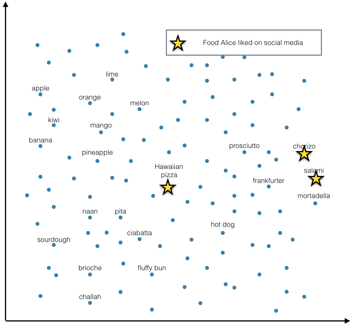
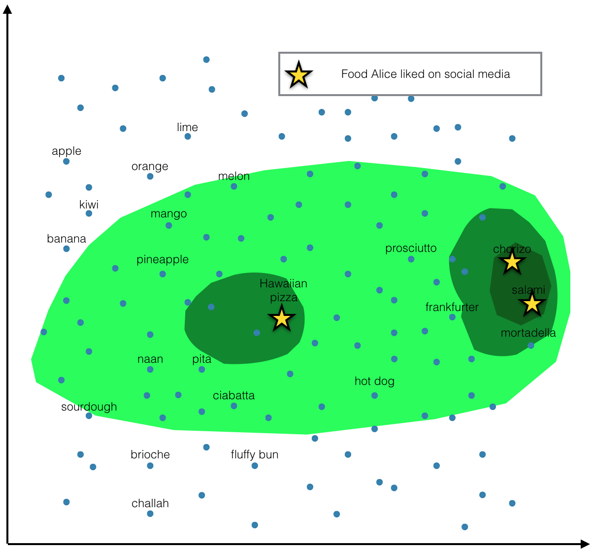
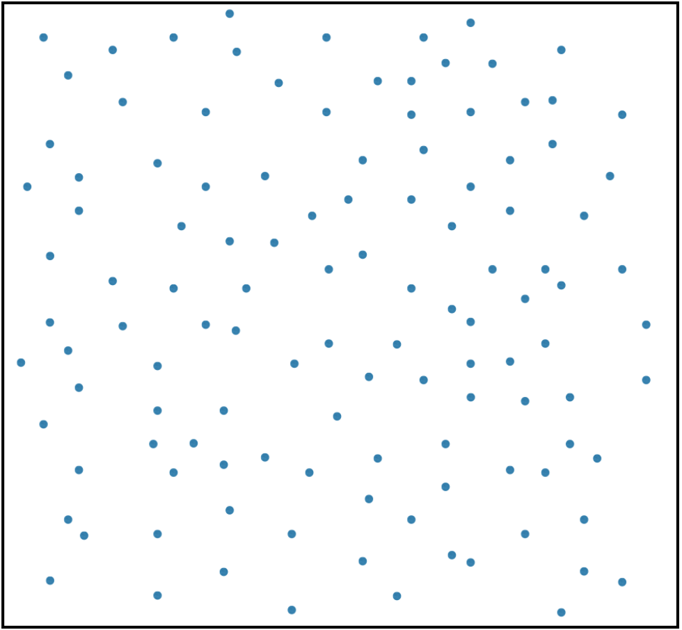
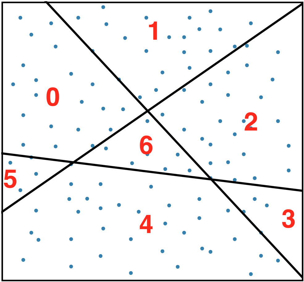
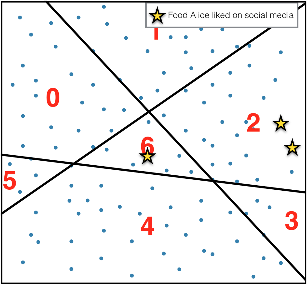
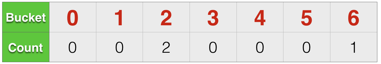
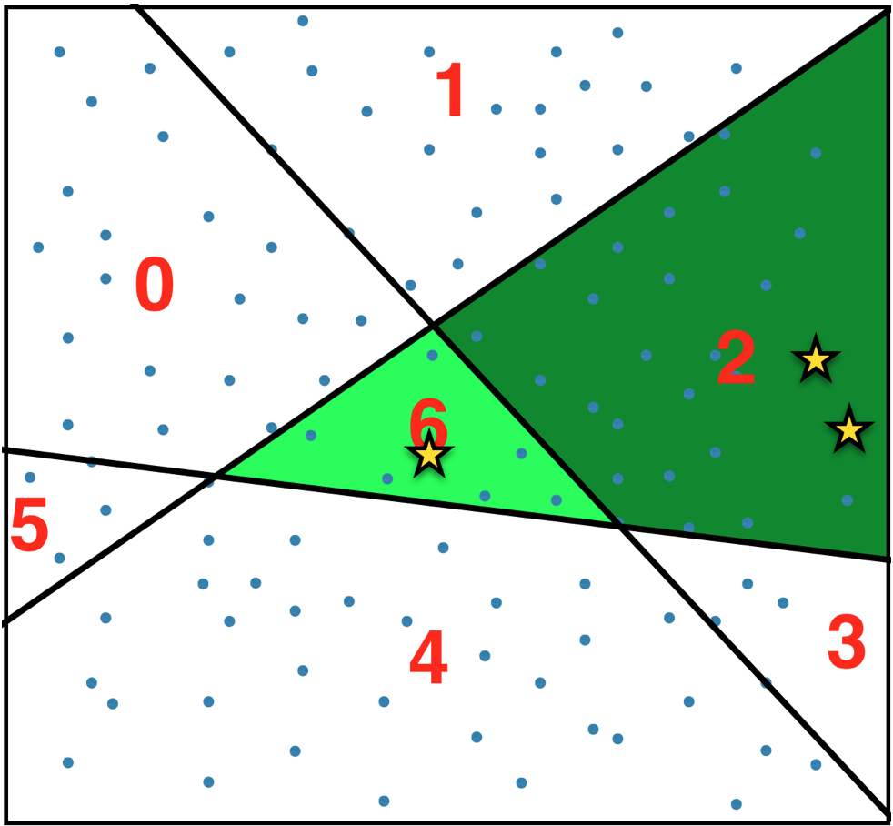
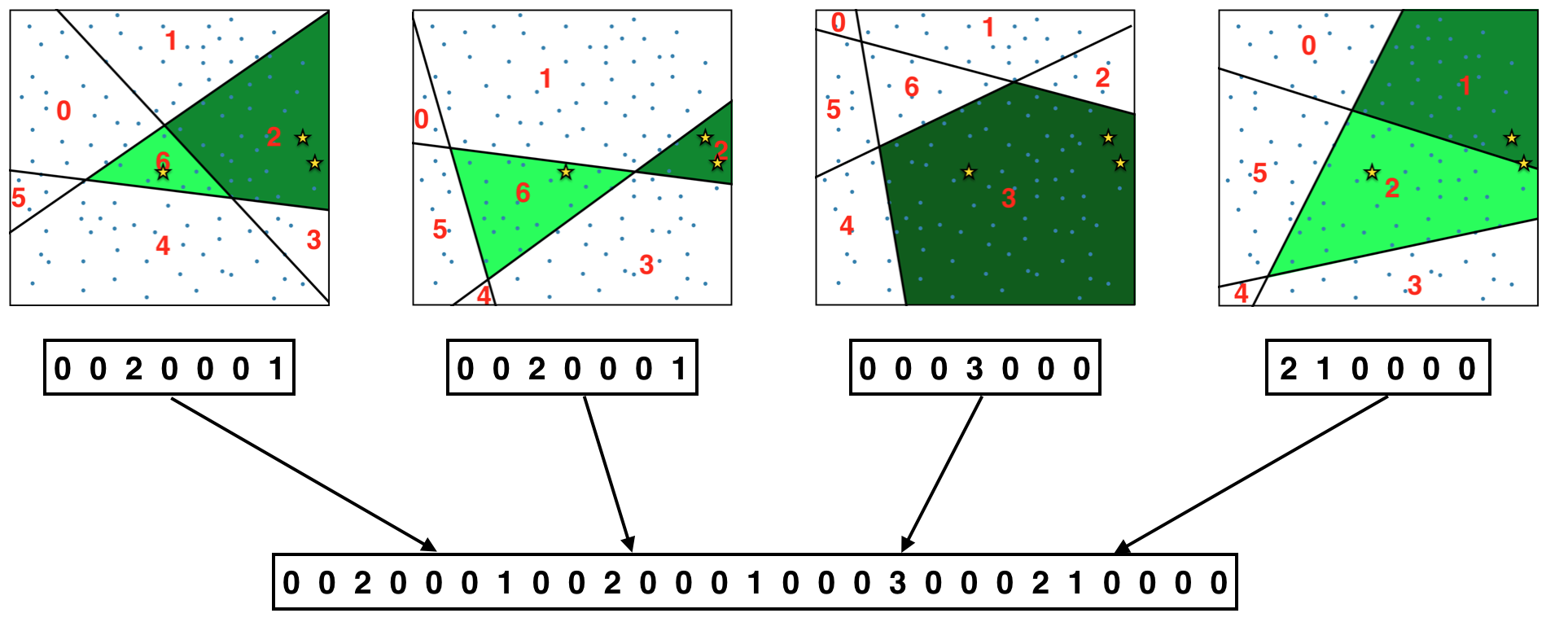
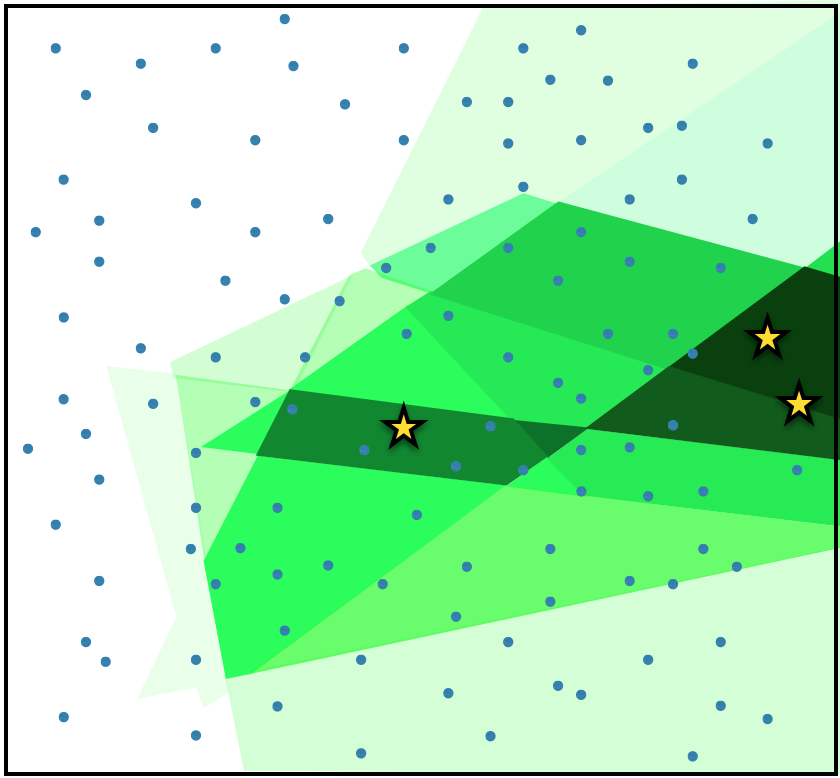
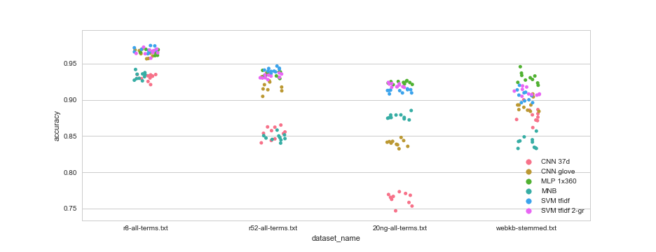
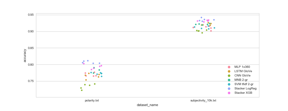

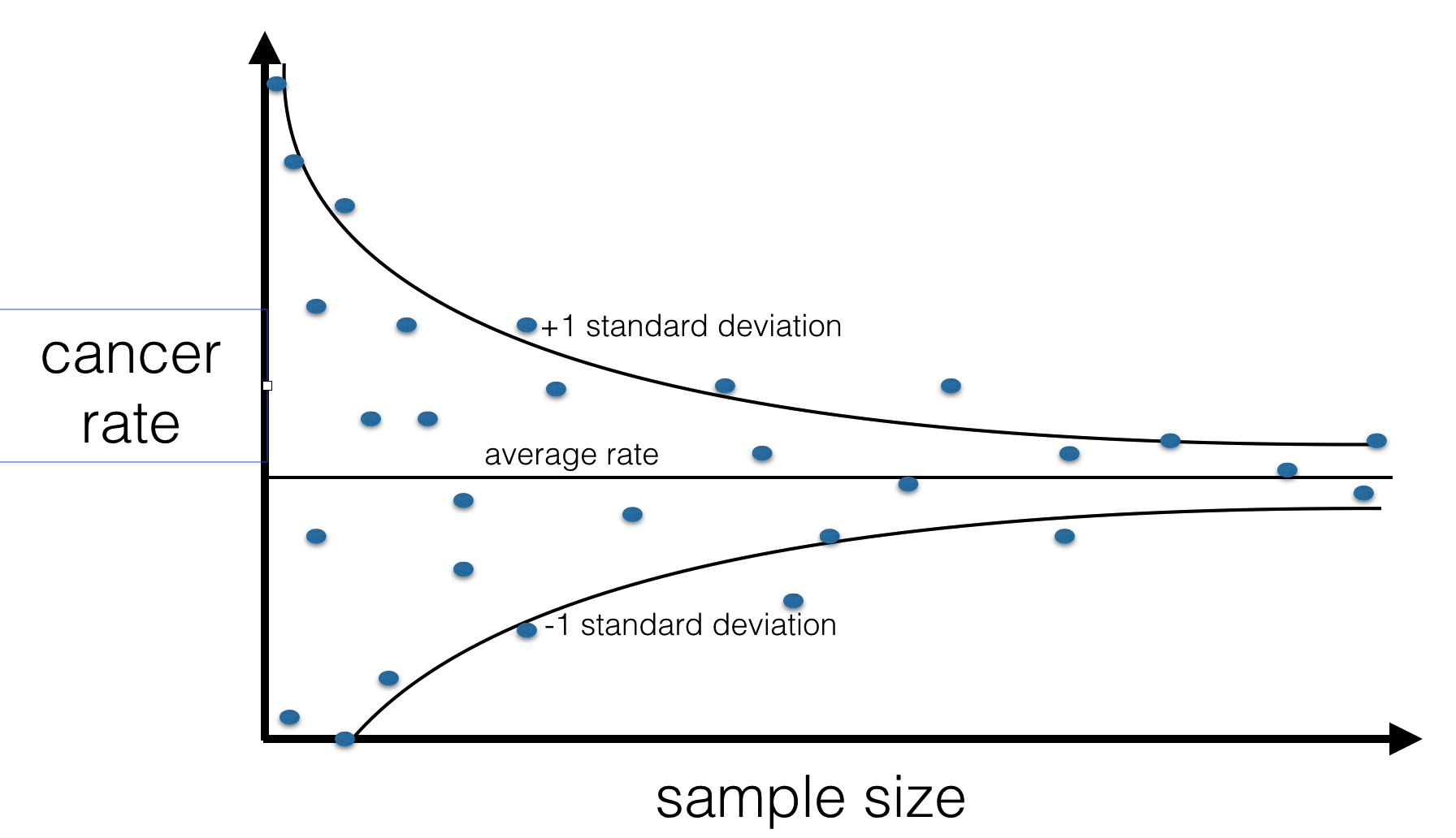
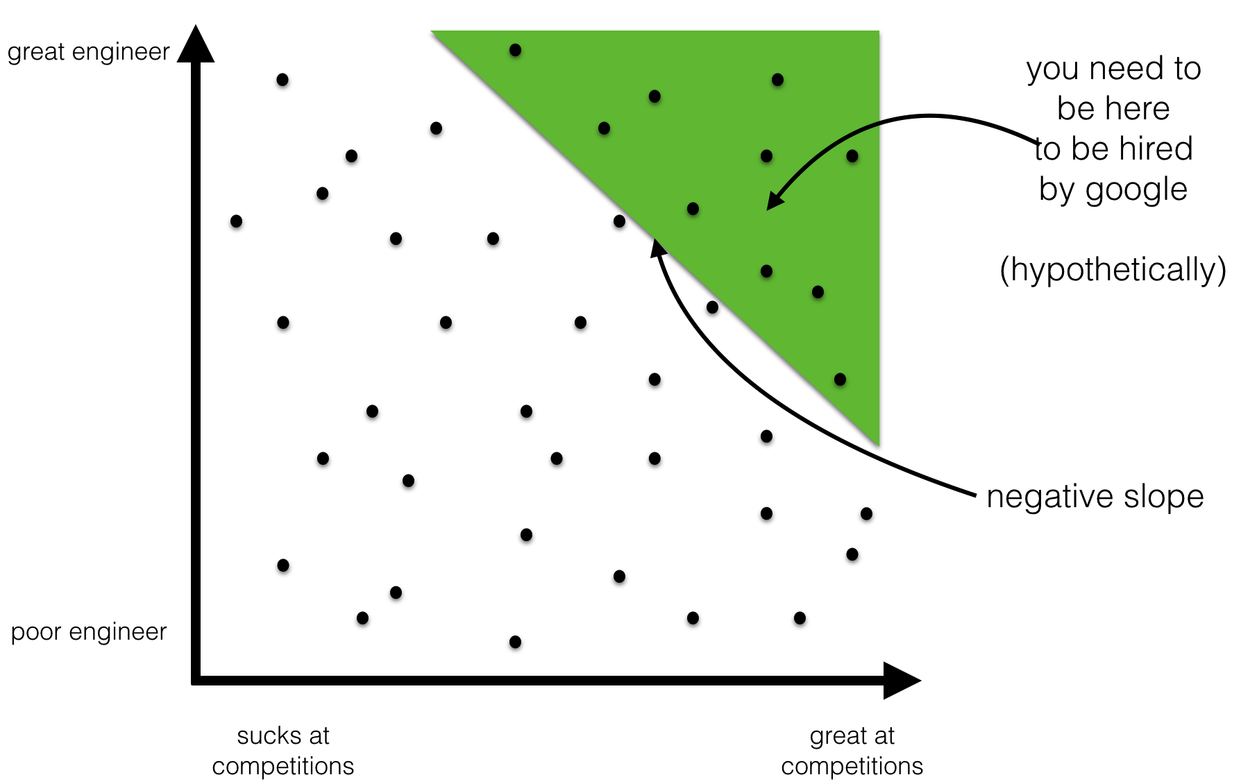
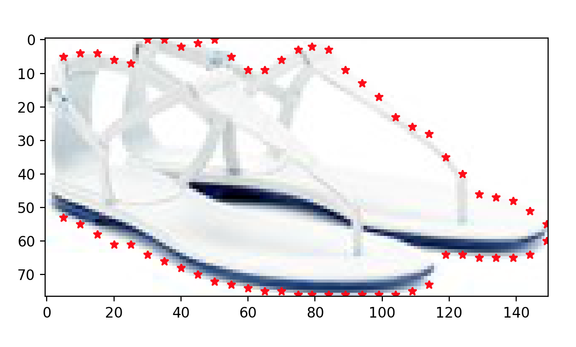
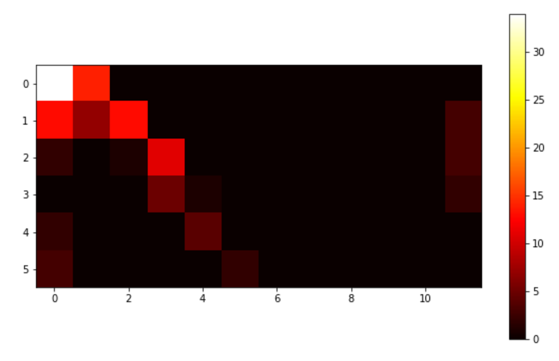
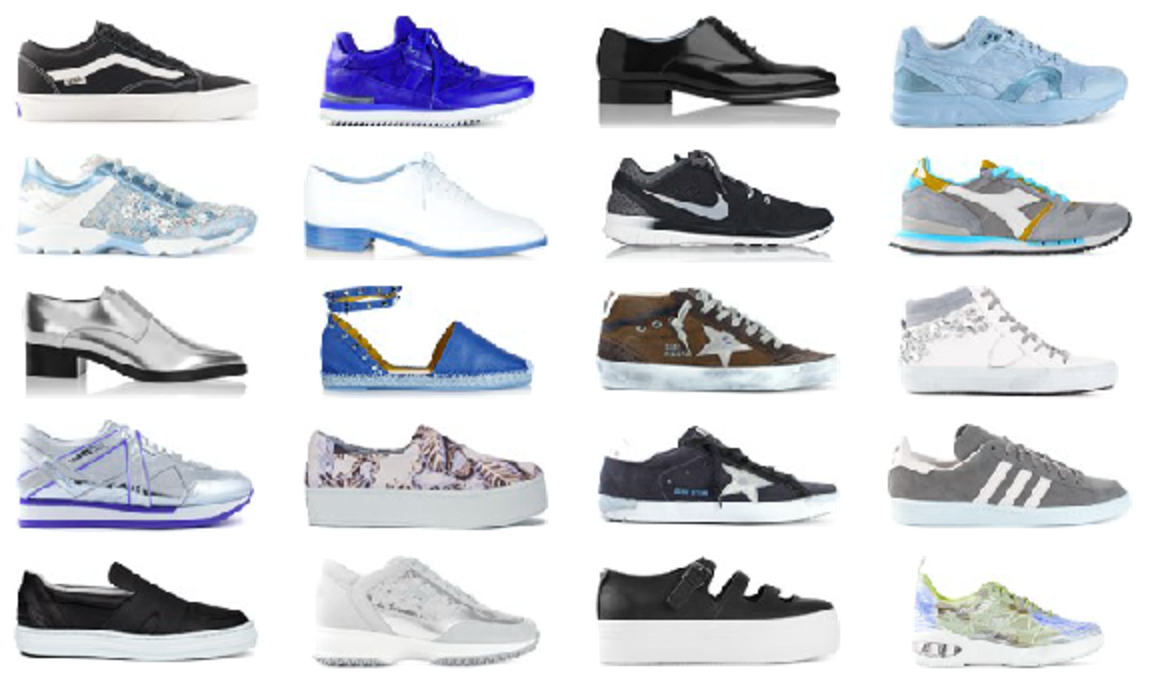

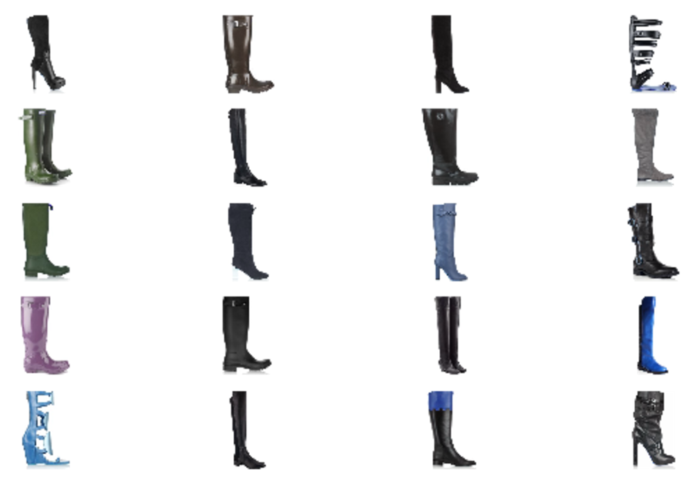
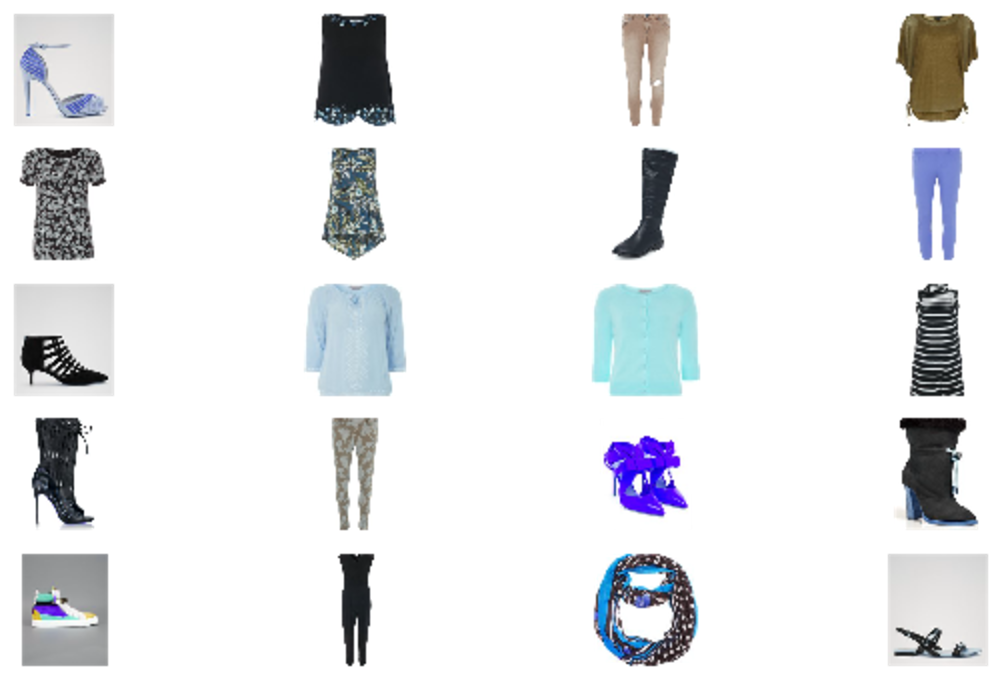