Missing Data Imputation With Bayesian Networks in Pymc

This is the first of two posts about Bayesian networks, pymc and missing data. In the first post I will show how to do Bayesian networks in pymc* and how to use them to impute missing data. This part is boring and slightly horrible. In the second post I investigate how well it actually works in practice (not very well) and how it compares to a more traditional machine learning approach (poorly). Feel free to go straight to the second post, it has plots in it.

This post assumes that the reader is already familiar with both bayesianism and pymc. If you aren’t, I recommend that you check out the fantastic Bayesian Methods For Hackers.

* technically, everything in pymc is a Bayesian network, I know

The problem

We have observed 10 animals and noted 3 things about each of them: - does it swim like a duck? - does it quack like a duck? - is it, in fact, a duck?

import pandas as pd

# we use 1 and 0 to represent True and False for reasons that will become clear later
full = pd.DataFrame({
    'swims_like_a_duck':  [0,0,0,0,1,1,1,1, 1, 1],
    'quacks_like_a_duck': [0,1,0,1,0,1,0,1, 0, 1],
    'duck':               [0,0,0,0,0,1,0,1, 0, 1]
})

It is easy to notice that in this dataset an animal is a duck if and only if it both swims like a duck and quacks like a duck. So far so good.

But what if someone forgets to write down whether the duck number 10 did any quacking or whether the animal number 9 was a duck at all? Now we have missing data. Here denoted by -1

with_missing = pd.DataFrame({
    'swims_like_a_duck':  [0,0,0,0,1,1,1,1,  1, -1],
    'quacks_like_a_duck': [0,1,0,1,0,1,0,1, -1, -1],
    'duck':               [0,0,0,0,0,1,0,1,  0,  1]
})

This tells us about the last animal that it is a duck, but the information about swimming and quacking is missing. Nevertheless, having established the rule

$(swims \: like \: duck) \land (quacks \: like \: duck) \Leftrightarrow (is \: duck)$

we can infer that the values of swims_like_a_duck and quacks_like_a_duck must both be 1 for this animal.

This is what we will try to do here - learn the relationship between the variables and use it to fill in the missing ones.

The Bayesian solution

To be able to attack this problem, let’s make one simplifying assumption. Let’s assume that we know the causal structure of the problem upfront. That is - we know that swimming and quacking are independent random variables, while being a duck is a random variable that potentially depends on the other two.

This is the situation described by this Bayesian network:

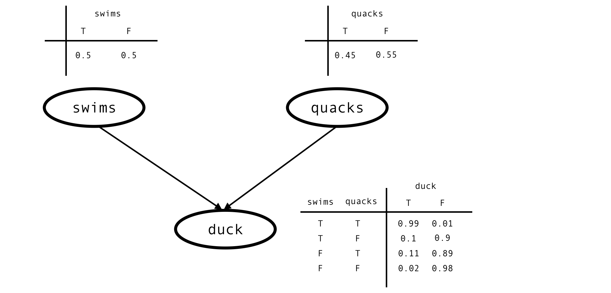
This network is fully characterised by 6 parameters - prior probabilities of swimming and quacking -
$P(swims)$, $P(quacks)$
- and conditional probability of being a duck given values of the other 2 variables -
$P(duck \mid swims \land quacks)$,
$P(duck \mid \neg swims \land quacks)$
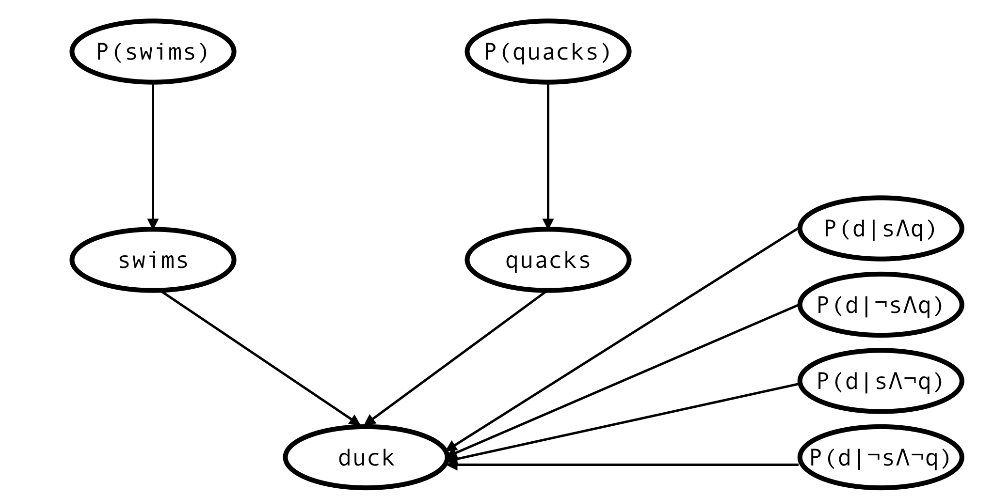
- and so on. We don’t know anything about the values of these parameters, other than they must be between $0$ and $1$. The bayesian thing to do in such situations is to model the unknown parameters as random variables of their own and give them uniform priors.

Thus, the network expands:

This is the network describing a single animal, but actually we have observations of many animals, so the full network would look more like this:

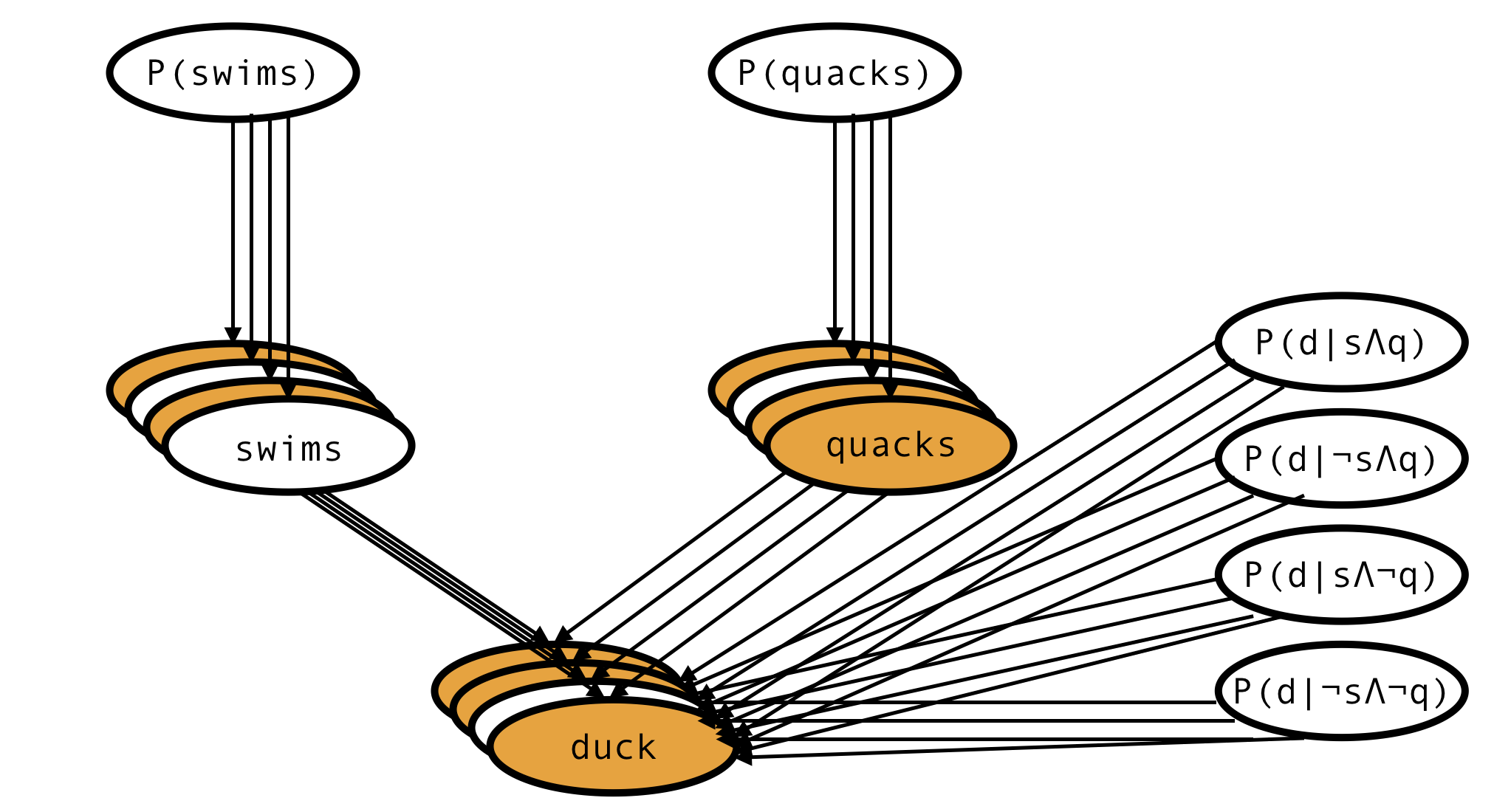
There is only one node corresponding to each of the 6 parameters, but there are as many ‘swims’ and ‘quacks’ and ‘duck’ nodes as there are records in the dataset.

Some of the variables are observed (orange), others aren’t (white), but we have specified priors for all the parent variables and the model is fully defined. This is enough to (via Bayes theorem) derive the formula for the posterior probability of every unobserved variable and the posterior distribution of every model parameter.

But instead of doing math, we will find a way to programmatically estimate all those probabilities with pymc. This way, we will have a solution that can be easily extended to arbitrarily complicated networks.

What could go wrong?

pymc implementation

Disclaimer: this is all hacky and inefficient in ways I didn’t realise it would be when I started working on it. pymc is not the right tool for the job, if you want to do this seriously, in a production environment you should look for something else. pymc3 maybe?

I will now demonstrate how to represent our quack-swim-duck Bayesian network in pymc and how to make predictions with it. pymc was confusing the hell out of me when I first started this project. I will be painstakingly explicit at every step of this tutorial to save the reader some of this confusion. Then at the end I will show how to achieve the same result with 1/10th as many lines of code using some utilities of my invention.

Let’s start with the unobserved variables:

import pymc
# prior probabilities for swimming and quacking
swim_prior = pymc.Uniform('P(swims)', lower=0, upper=1, size=1)
quack_prior = pymc.Uniform('P(quacks)', lower=0, upper=1, size=1)

# probability of being a duck conditional on swimming and quacking
# (or not swimming and quacking etc.)
p_duck_swim_quack = pymc.Uniform('P(duck | swims & quacks)', lower=0, upper=1, size=1)
p_duck_not_swim_not_quack = pymc.Uniform('P(duck | not swims & not quacks)', lower=0, upper=1, size=1)
p_duck_not_swim_quack = pymc.Uniform('P(duck | not swims & quacks)', lower=0, upper=1, size=1)
p_duck_swim_not_quack = pymc.Uniform('P(duck | swims & not quacks)', lower=0, upper=1, size=1)

Now the observed variables. pymc requires that we use masked arrays to represent missing values:

import numpy as np
swim_data = with_missing.swims_like_a_duck
masked_swim_data = np.ma.masked_array(swim_data, swim_data == -1, fill_value=0)

quack_data = with_missing.quacks_like_a_duck
masked_quack_data = np.ma.masked_array(quack_data, quack_data == -1, fill_value=0)

duck_data = with_missing.duck
masked_duck_data = np.ma.masked_array(duck_data, duck_data == -1, fill_value=0)

This is what a masked array with two missing values looks like:

>>> masked_quack_data
masked_array(data = [0 1 0 1 0 1 0 1 -- --],
             mask = [False False False False False False False False  True  True],
       fill_value = 0)

Quacking and swimming nodes:

# number of animal observations
n = len(with_missing)

# with 'size=n' with tell pymc that 'swims' is actually a sequence of n Bernoulli variables
swims = pymc.Bernoulli('swims', p=swim_prior, observed=True, value=masked_swim_data, size=n)
quacks = pymc.Bernoulli('quacks', p=quack_prior, observed=True, value=masked_quack_data, size=n)

And now the hard part. We have to construct a Bernoulli random variable ‘duck’, whose conditional probability given its parents is equal to a different random variable for very combination of values of the parents. That was a mouthful, but all it means is that there is a conditional probability table of ‘duck’ conditioned on ‘swims’ and ‘quacks’. This is literally the first example in every textbook on probabilistic models. And yet, there is no easy way to express this relationship with pymc. We are forced to roll our own custom function.

# auxiliary pymc variable - probability of duck
@pymc.deterministic
def duck_probability(
        swims=swims,
        quacks=quacks,
        p_duck_swim_quack=p_duck_swim_quack,
        p_duck_not_swim_quack=p_duck_not_swim_quack,
        p_duck_swim_not_quack=p_duck_swim_not_quack,
        p_duck_not_swim_not_quack=p_duck_not_swim_not_quack):

    d = []
    for s, q in zip(swims, quacks):
        if (s and q):
            d.append(p_duck_swim_quack)
        elif (s and (not q)):
            d.append(p_duck_swim_not_quack)
        elif ((not s) and q):
            d.append(p_duck_not_swim_quack)
        elif ((not s) and (not q)):
            d.append(p_duck_not_swim_not_quack)
        else:
            raise ValueError('this should never happen')

    return np.array(d).ravel()

# AND FINALLY
duck = pymc.Bernoulli('duck', p=duck_probability, observed=True, value=masked_duck_data, size=n)

If you’re half as confused reading this code as I was when I was first writing it, you deserve some explanations.

‘swims’ and ‘quacks’ are of type pymc.distributions.Bernoulli, but here we treat them like numpy arrays.

This is @pymc.deterministic’s doing. This decorator ensures that when this function is actually called it will be given swims.value and quacks.value as parameters - and these are indeed numpy arrays. Same goes for all the other parameters.

earlier we used a pymc random variable for the p parameter of a pymc.Bernoulli but now we’re using a function - duck_probability

Again, @pymc.deterministic. When applied to a function it returns an object of type pymc.PyMCObjects.Deterministic. At this point the thing bound to the name ‘duck_probability’ is no longer a function. It’s a pymc random variable. It has a value parameter and everything.

Ok, let’s put it all together in a pymc model:

# putting it all together
model = pymc.Model([swims, quacks, duck])

aaaand we’re done.

Not really. The network is ready, but there is still the small matter of extracting predictions out of it.

Making predictions with MAP

The obvious way to estimate the missing values is with a maximum a posteriori estimator. Thankfuly, pymc has just the thing - pymc.MAP. Calling .fit on a pymc.MAP object changes values of variables in place, so let’s print the values of some of our variables before and after fitting.

>>> print swims.value
[False False  True  True False False  True  True  True False]
>>> print quacks.value
[False  True False  True False  True False  True False False]
>>> print duck.value
[False False False  True False False False  True False  True]
>>> print swim_prior.value
[ 0.58298865]
>>> print quack_prior.value
[ 0.58990097]
>>> print p_duck_not_swim_quack.value
[ 0.96976671]
>>> print p_duck_swim_quack.value
[ 0.12251178]

optimise the values:

>>> pymc.MAP(model).fit()
Warning: Stochastic swims's value is neither numerical nor array with floating-point dtype. Recommend fitting method fmin (default).

and inspect the results:

>>> print swims.value
[False False  True  True False False  True  True  True  True]
>>> print quacks.value
[False  True False  True False  True False  True False  True]
>>> print duck.value
[False False False  True False False False  True False  True]
>>> print swim_prior.value
[ 0.6]
>>> print quack_prior.value
[ 0.5]
>>> print p_duck_not_swim_quack.value
[  9.42288677e-10]
>>> print p_duck_swim_quack.value
[ 0.99999999]

The two False bits - in ‘swims’ and ‘quacks’ have flipped to True and the values of the conditional probabilities have moved in the right direction! This is good, but unfortunately it’s not reliable. Even in this simple example pymc’s MAP rarely gets everything right like it did this time. To some extent it depends on the optimisation method used - e.g. pymc.MAP(model).fit(method='fmin') vs pymc.MAP(model).fit(method='fmin_powell'). Despite the warning message recommending ‘fmin’, ‘fmin_powell’ gives better results. ‘fmin’ gets the (more or less) right values for continous parameters but it never seems to flip the booleans, even when it would clearly result in higher likelihood.

Making predictions with MCMC

The other way of getting predictions out of pymc is to use it’s main workhorse - the MCMC sampler. We will generate 200 samples from the posterior using MCMC and for each missing value we will pick the value that is most frequent among the samples. Mathematically this is still just maximum a posteriori estimation but the implementation is very different and so are the results.

# this will generate (10000 - 8000) / 10 = 200 samples
sampler = pymc.MCMC(model)
sampler.sample(iter=10000, burn=8000, thin=10)

This should have produced 200 samples from the posterior for each unobserved variable. To see them, we use sampler.trace.

>>> sampler.trace('P(swims)')[:].shape
(200, 1)

200 samples of the 'P(swims)' paramter - as promised

>>> sampler.trace('P(duck | not swims & quacks)')[:].shape
(200, 1)

200 samples of a conditional probability parameter.

>>> sampler.trace('swims')[:].shape
(200, 1)

swims boolean variable also has 200 samples. But:

>>> sampler.trace('quacks')[:].shape
(200, 2)

quacks has two times 200 - because there were two missing values among quacks observations - and each is modeled as an unobserved variable.

sampler.trace('duck') produces only a KeyError - there are no missing values in duck, hence no samples.

Finally, posterior probability for the missing swims observation:

>>> sampler.trace('swims')[:].mean(axis=0)
array([ 0.62])

Great! According to MCMC the missing value in swims is more likely than not to be True!

(sampler.trace('swims')[:] is an array of 200 booleans, counting the number of True and False is equivalent to simply taking the mean).

>>> sampler.trace('quacks')[:].mean(axis=0)
array([ 0.195,  0.6  ])

And the two missing values in quacks are predicted to be False and True - respectively. As they should be.

Unlike the MAP approach, this result is reliable. As long as you give MCMC enough iterations to burn in, you will get very similar numbers every time.

The clean way

This was soul-crushingly tedious, I know. But it doesn’t have to be this way. I have created a few utility functions to get rid of the boilerplate - the creation of uniform priors for variables, the conditional probabilities, the trace, and so on. The utils can all be found here (along with some other stuff).

This is how to define the network using these utils:

from dstk.pymc_utils import make_bernoulli, cartesian_bernoulli_child
from dstk.imputation import BayesNetImputer

class DuckImputer(BayesNetImputer):
    def construct_net(self, df):
        quacks = make_bernoulli('quacks_like_a_duck', value=df.quacks_like_a_duck)
        swims = make_bernoulli('swims_like_a_duck', value=df.swims_like_a_duck)
        duck = cartesian_bernoulli_child('duck', parents=[quacks, swims], value=df.duck)
        return pymc.Model([quacks, swims, duck])

(there are also versions of make_bernoulli and cartesian_bernoulli_child for categorical variables). And this is how to use it:

>>> print DuckImputer(method='MCMC').fit_transform(with_missing)
    duck  quacks_like_a_duck  swims_like_a_duck
   0                   0                  0
   0                   1                  0
   0                   0                  1
   1                   1                  1
   0                   0                  0
   0                   1                  0
   0                   0                  1
   1                   1                  1
   0                   0                  1
   1                   0                  1

Next post: how all this compares to good old xgboost.

DS lore

words about stuff