In the last post I presented a way to do Bayesian networks with pymc and use them to impute missing data. This time I benchmark the accuracy of this method on some artificial datasets.

Datasets

In the previous posts I showed the imputation of boolean missing data, but the same method works for categorical features of any cardinality as well as continuous ones (except in the continues case additional prior knowledge is required to specify the likelihood). Nevertheless, I decided to test the imputers on purely boolean datasets because it makes the scores easy to interpret and the models quick to train.

To make it really easy on the Bayesian imputer, I created a few artificial datasets by the following process:

1. define a Bayesian network
2. sample variables corresponding to conditional probabilities describing the network from their priors (once)
3. fix the parameters from step 2. and sample the other variables (the observed ones) repeatedly

With data generated by the same Bayesian network that we will fit to it, we’re making it as easy on pymc as possible to get a good score. Mathematically speaking, the bayesian model is the way to do it. Anything less than optimal performance can only be due to a bug or pymc underfitting (perhaps from too few iterations).

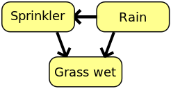
The first dataset used is based on the famous wet sidewalk - rain - sprinkler network as seen in the wikipedia article on Bayesian networks.

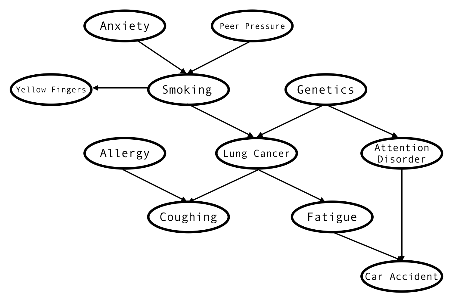
The second, bigger, is based on the LUCAS network

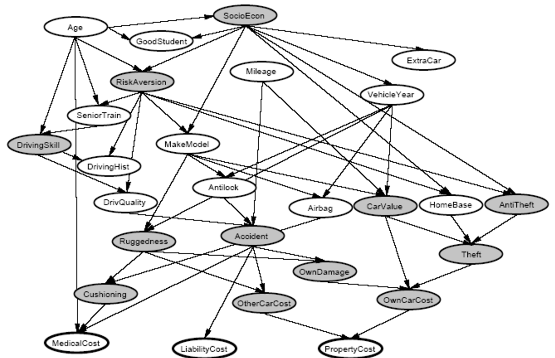
And the biggest one is based on an example from some ML lecture notes

For each of these networks I would generate a dataframe with 10, 50, 250, 1250 or 6250 records and drop (replace with -1) a random subset of 20% or 50% of values in each column. Then I would try to fill them in with each model and score the model on accuracy. This was repeated 5 times for each network and data size and the accuracy reported is the mean of the 5 tries.

Models

The following models were used to impute the missing records:

• most frequent - a dummy model that predicts most frequent value per dataframe column. This is the absolute baseline of imputer performance, every model should be at least as good as this.
• xgboost - a more ambitious machine learning-based baseline. This imputer simply trains an XGBoost Classifier for every column of the dataframe. The classifier is trained only on the records where the value of that column is not missing and it uses all the remaining columns to predict that one. So, if there are n columns - n classifiers are trained, each using n - 1 remaining columns as features.
• MAP fmin_powell - a model constructed the same way as the DuckImputer model from the previous post. Actually, it’s a different model for each dataset, but the principle is the same. You take the very same Bayesian network that was used to create the dataset and fit it to the dataset. Then you predict the missing values using MAP with ‘method’ parameter set to ‘fmin_powell’.
• MAP fmin - same as above, only with ‘method’ set to ‘fmin’. This one actually performed so poorly, (no better than random and worse than most frequent) and was so slow that I quickly dropped it from the benchmark
• MCMC 500, MCMC 2000, MCMC 10000 - same as the MAP models, except for the last step. Instead of finding maximum a posteriori for each variable directly using the MAP function, the variable is sampled n times from the posterior using MCMC, and the empirically most common value is used as the prediction. Three versions of this model were used - with 500, 2000 and 10000 iterations for burn-in repectively. After burn-in, 200 samples were used each time.

Results

Let’s start with the simplest network:

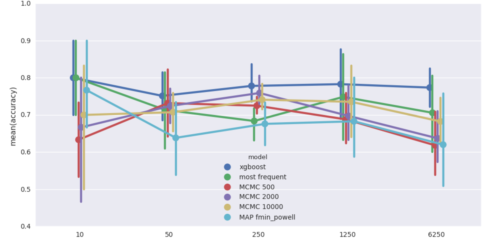Rain-Sprinkler-Wet Sidewalk benchmark (20% missing values). Mean imputation accuracy from 5 runs vs data size.

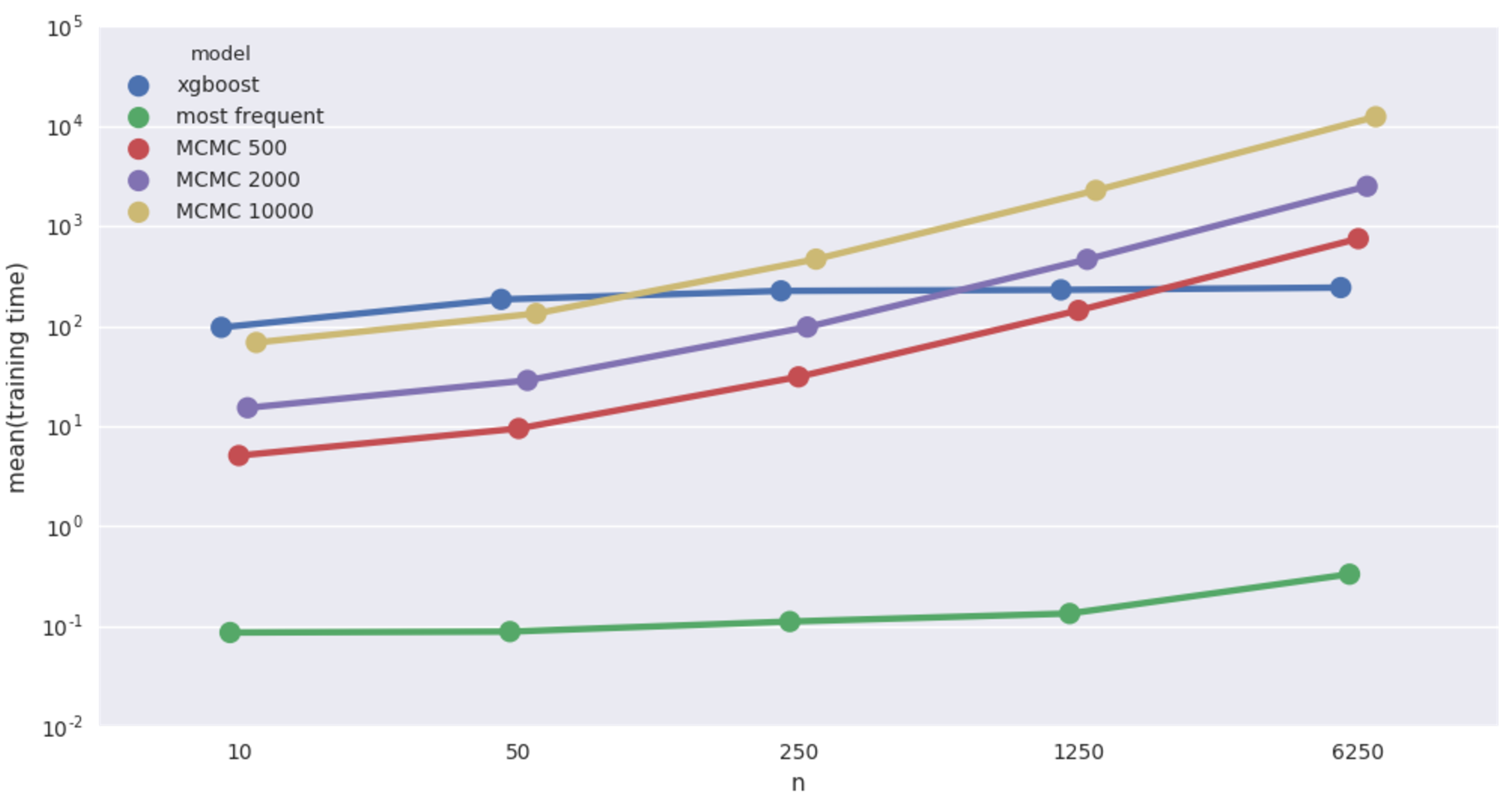
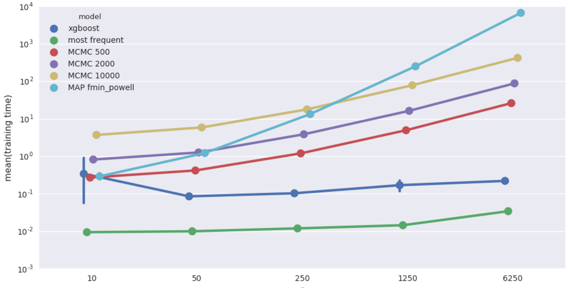Average fitting time in seconds. Beware log scale!

XGBoost comes out on top, bayesian models do poorly, apparently worse than even most frequent imputer. But variance in scores is quite big and there is not much structure in this dataset anyway, so let’s not lose hope. MAP fmin_powell is particularly bad and terribly slow on top of that, dropping it from further benchmarks.

Let’s try a wider dataset - the cancer network. This one has more structure - that the bayesian network knows up front and xgboost doesn’t - which should give bayesian models an edge.

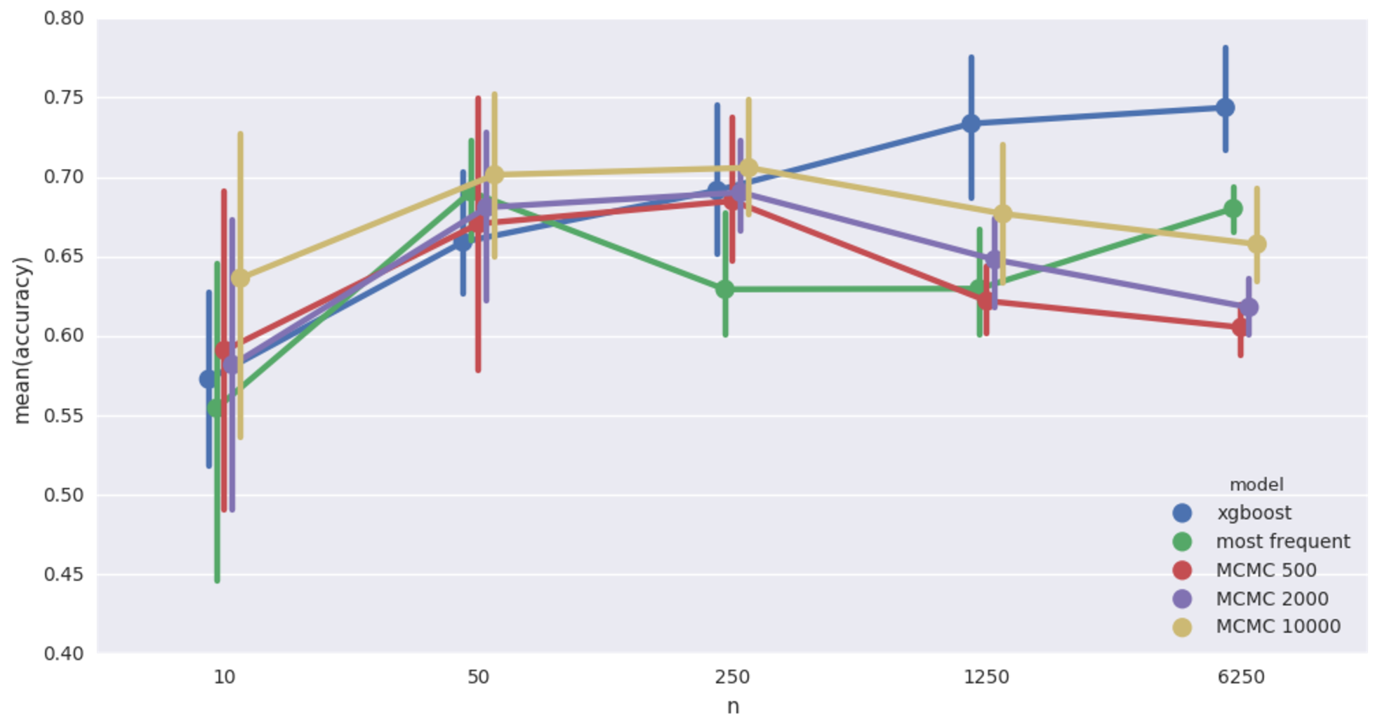Cancer network imputation accuracy. 20% missing values

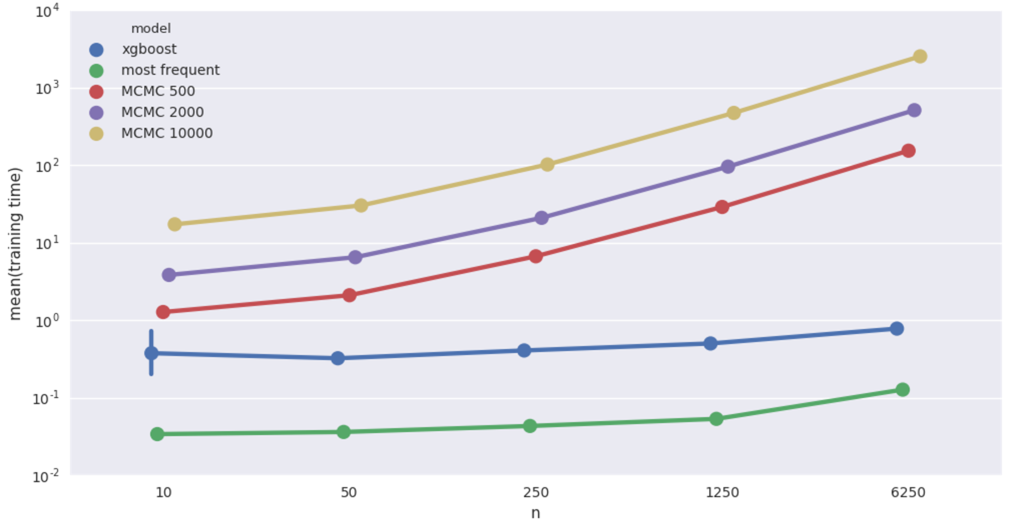Cancer network imputation time.

That’s more like it! MCMC wins when records are few, but deteriorates when data gets bigger. MCMC models continue to be horribly slow.

And finally, the biggest (27 features!), car insurance network.

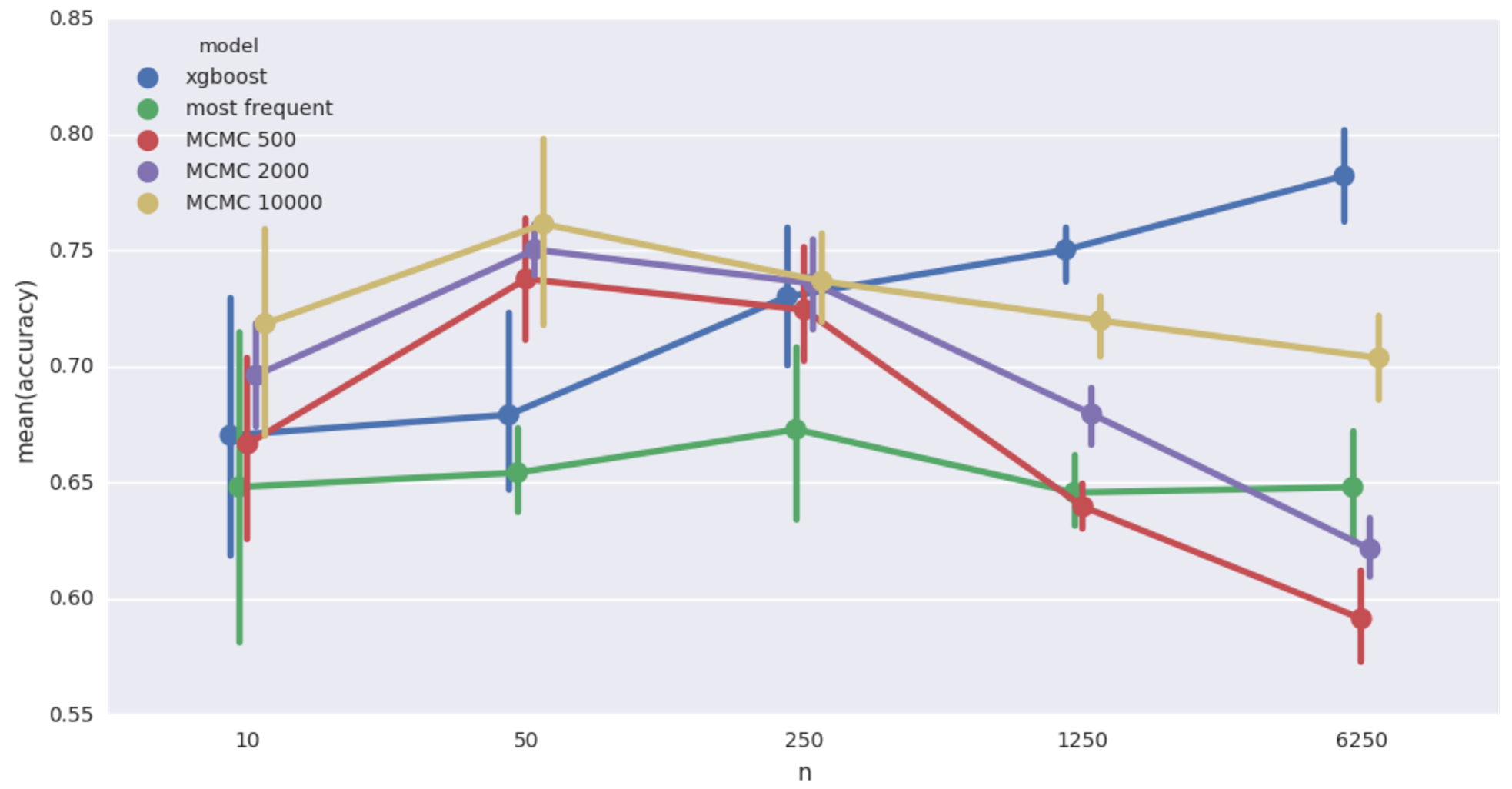Car insurance network imputation accuracy. 20% missing values

Car insurance network imputation time.

Qualitatively same as the cancer network case. It’s worth pointing out that in this case, the Bayesian models achieve at 50 records a level of accuracy that XGBoost doesn’t match until shown more than a thousand records! Still super slow though.

Conclusions

What have we learned?

1. Bayesian models do relatively better when data is wide (more columns). This was expected. Wide data means bigger network, means there is more information implicit in the network structure. This is information that we hardcode into the Bayesian model, information that XGBoost doesn’t have.
2. Bayesian models do relatively better when data is short (less records). This was also expected, for the same reason. When data is short, the information contained in the network counts for a lot. With more records to train on, this advantage gets less important.
3. pymc’s MAP does poorly in terms of accuracy and is terribly slow, slower than MCMC. This one is a bit of a mystery.
4. For MCMC, longer burn-in gets better results, but takes more time. Duh.
5. MCMC model accuracy deteriorates as data gets bigger. I was surprised when I saw it, but it hindsight it’s clear that it would be the case. Bigger data means more missing values, means higher dimensionality of the space MCMC has to explore, means it would take more iterations for MCMC to reach a high likelihood configuration. This could be alleviated if we first learned the most likely values of the parameters of the network and then used those to impute the missing values one record at a time.
6. XGBoost rocks.

Overall, I count this experiment as a successful proof of concept, but of very limited usefulness in its current form. For any real world application one would have to redo it using some other technology. pymc is just not up to the task.