This is a guest post by Javier Rodriguez Zaurin.

My good friend Nadbor told me that he found on Reddit someone asking if data scientists end up doing boring tasks such as classifying shoes. As someone that has faced this problem in the past, I was committed to show that classifying shoes it is a challenging, entertaining task. Maybe the person who wrote that would find it more interesting if the objects to classify were space rockets, but whether rockets or shoes, the problem is of the same nature.

THE PROBLEM

Imagine that you work at a fashion aggregator, and every day you receive hundreds of shoes in the daily feed. The retailers send you one identifier and multiple images (with different points of view) per shoe model. Sometimes, they send you additional information indicating whether one of the images is the default image to be displayed at the site, normally, the side-view of the shoe. However, this is not always the case. Of course, you want your website to look perfect, and you want to consistently show the same shoe perspective across the entire site. Therefore, here is the task: how do we find the side view of the shoes as they come through the feed?

THE SOLUTION

Before I jump into the technical aspect of the solution, let me just add a few lines on team-work. Through the years in both real science and data science, I have learned that cool things don’t happen in isolation. The solution that I am describing here was part of a team effort and the process was very entertaining and rewarding.

Let’s go into the details.

The solution implemented comprised two steps:

1-. Using the shape context algorithm to parameterise shoe-shapes

2-. Cluster the shapes and find those clusters that are comprised mostly by side-view shoes

THE SHAPE CONTEXT ALGORITHM

Details on the algorithm can be found here and additional information on our python implementation is here. The steps required are mainly two:

1-. Find points along the silhouette of the shoe useful to define the shape.

2-. Compute a Shape Context Matrix using radial and angular metrics that will effectively parameterise the shape of the shoe.

1-. FIND THE RELEVANT POINTS

Finding the relevant points to be used later to compute the Shape Context Matrix is relatively easy. If the background of the image is white, simply “slice” the image and find the initial and final points that are not background per slice. Note that due to the “convoluted” shapes of some shoes, techniques relying on contours might not work here.

I have coded a series of functions to make our lives easier. Here I show the results of using some of those functions.

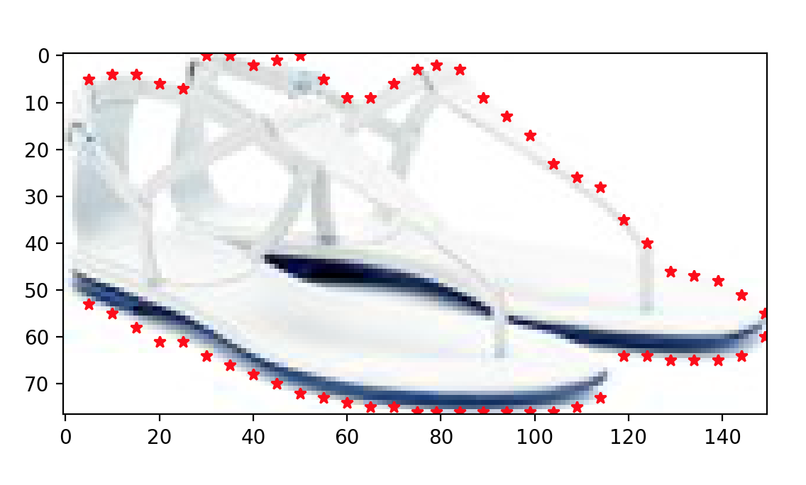
The figure shows 60 points of interest found as we move along the image horizontally.

2-. SHAPE CONTEXT MATRIX

Once we have the points of interest we can compute the radial and angular metrics that will eventually lead to the Shape Context Matrix. The idea is the following: for a given point, compute the number of points that fall within a radial bin and an angular bin relative to that point.

In a first instance, we computed 2 matrices, one containing radial information and one containing angular information, per point of interest. For example, if we select 120 points of interest around the silhouette of the shoe, these matrices will be of dim (120,120).

Once we have these matrices, the next step consists in building the shape context matrix per point of interest. Eventually, all shape context matrices are flattened and concatenated resulting in what is referred to as Bin Histogram.

Let’s have a look at one of these shape context matrices. For this particular example we used 6 radial bins and 12 angular bins. Code to generate this plot can be found here:

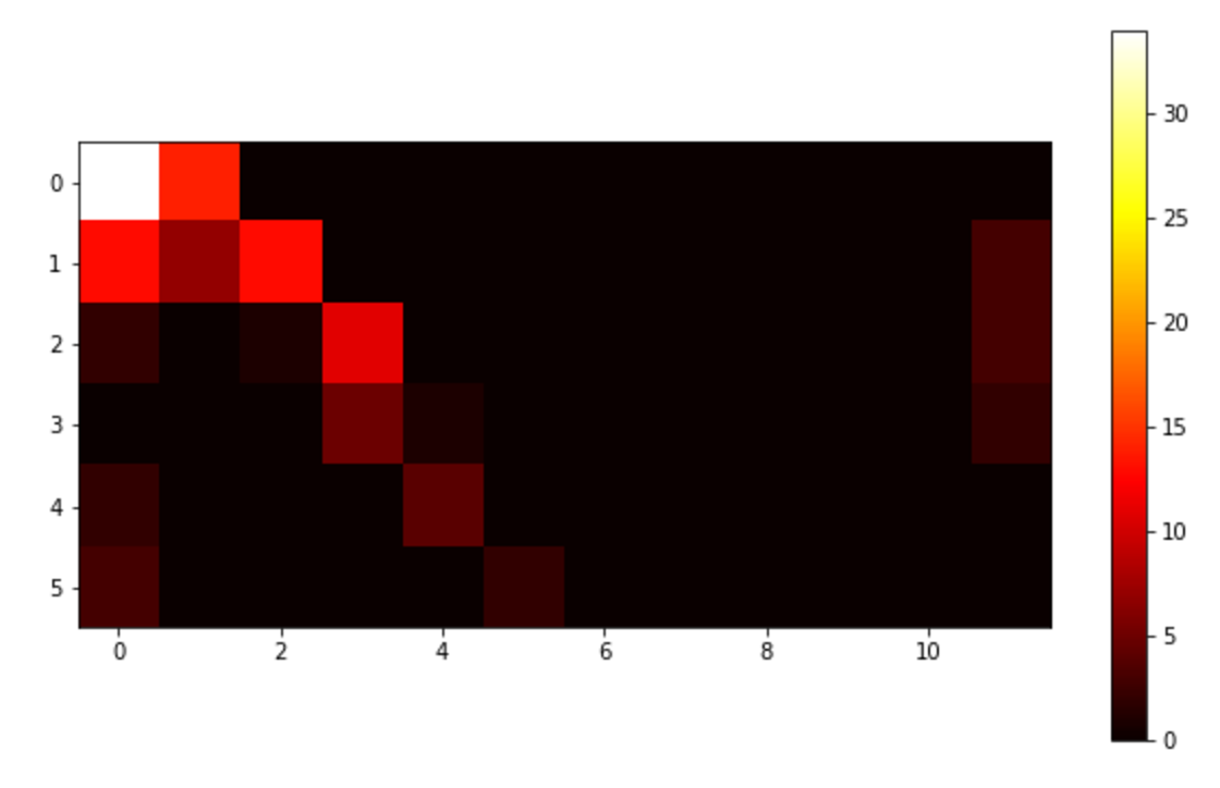
This figure has been generated for the first point within our points-of-interest-array and is interpreted as follows: if we concentrate on the upper-left “bucket” we find that, relative to the first point in our array, there are 34 other points that fall within the largest radial bin (labelled 0 in the Figure) and within the first angular bin (labelled 0 in the Figure). More details on the interpretation can be found here

Once we have a matrix like the one in Figure 2 for every point of interest, we flatten and concatenate them resulting in an array of 12 $\times$ 6 $\times$ number of points (120 in this case), i.e. 8640 values. Overall, after all this process we will end up with a numpy array of dimensions (number of images, 8640). Now we just need to cluster these arrays.

RESULTS

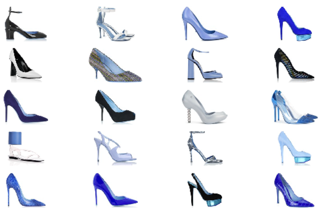
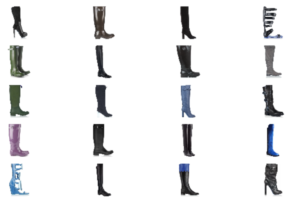
A detailed discussion on how to pick the number of clusters and the potential caveats can be found here. In this post I will simply show the results of using MiniBatchKMeans to cluster the arrays using 15 clusters. For example, clusters 2,3 and 10 look like this.

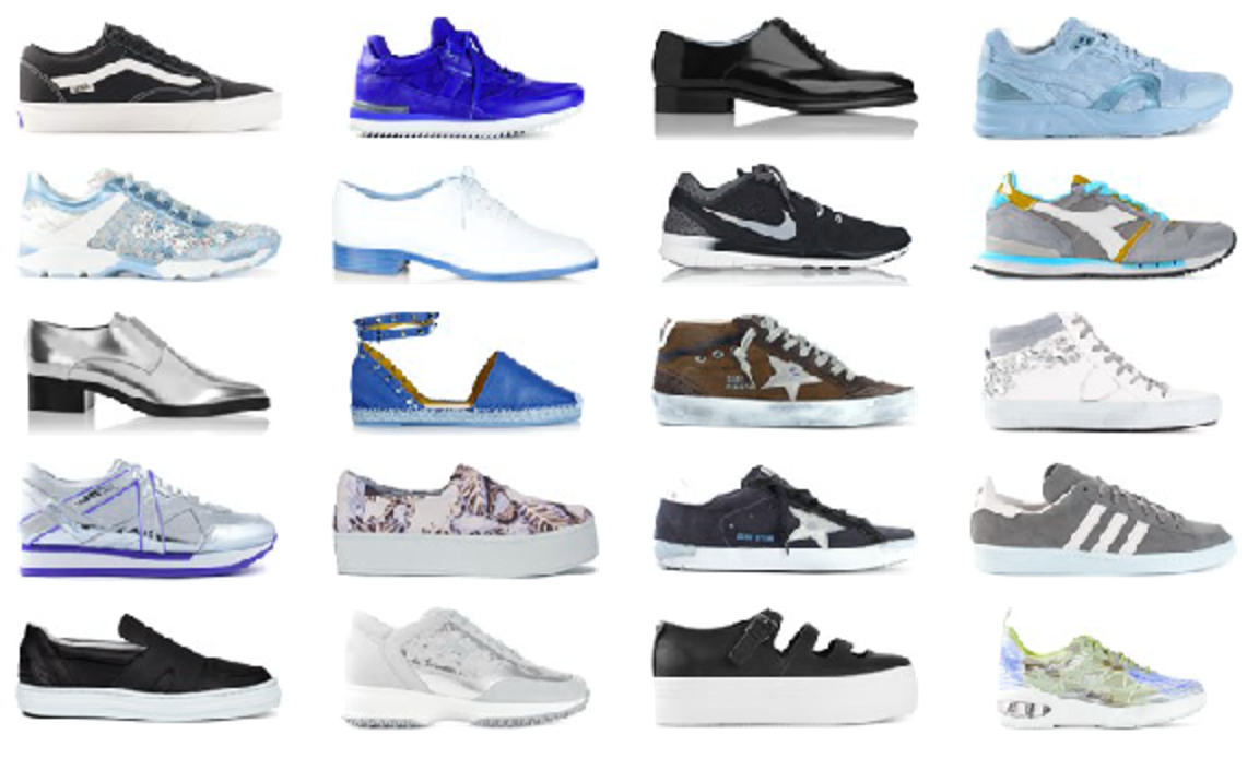
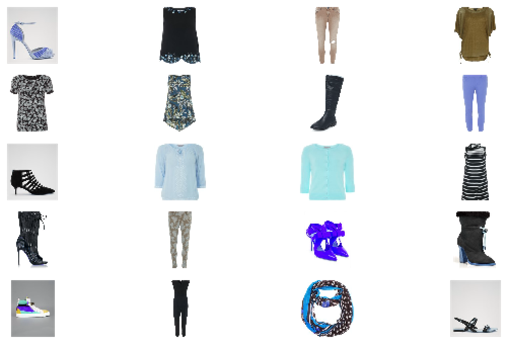
Interestingly cluster 1 is comprised of images with an non-white and/or structured background, images with a shape different than that of a shoe and some misclassifications. Some advise on how to deal with the images in that cluster can be found here

MOVING FORWARD

There are still a few aspects to cover to isolate the side views of the shoes with more certainty, but I will leave this for a future post (if I have the time!).

In addition, there are some other features and techniques one could try to improve the quality of the clusters, such as GIST indicators or Halarick Textural Features.

Of course, if you have the budget, you can always pay for someone to label the entire dataset, turn this into a supervised problem and use Deep Learning. A series of convolutional layers should capture shapes, colours and patterns. Nonetheless, if you think for a second about the nature of this problem, you will see that even deciding the labelling is not a trivial task.

Anyway, for now, I will leave it here!

The code for the process described in this post can be found here